книги / Разработка нефтяных и газовых месторождений

where P2 is terminal oil pipeline pressure; ∆Z is difference between geometric

(elevation) marks	of the beginning and end of	oil pipeline:	∆Z = Z2 − Z1 .	At
Z2 > Z1 magnitude	∆Z should be taken with (+)	sign, and at	Z2 < Z1 – with	(–)

sign. Elevations of some sections of oil pipeline can exceed Z2 ( Z2 > Z1 ), and they should be considered in filling oil pipeline with fluid.

7.3. Gas Pipeline Hydraulic Calculation

The distinguishing feature of gas flow in gas pipeline is gas volume changing due to real gas compressibility and supercompressibility. Volumetric gas flow velocity becomes higher as pressure becomes lower, what causes friction pressure drop per unit of pipeline length. Volumetric flow rate or gas pipeline throughput capacity can be determined by the below formula (for new pipes):

Q = 0,417 D	8 / 3	P2 − P2			3	(15)
		ρ	L T	Z , m /sec,
		1	2

отн

where D is inside pipe diameter; L is length of gas pipeline; P1 and P2 are, respectively, gas pipeline admission pressure and terminal gas pipeline pressure; T is average gas temperature in gas pipeline; ρотн is relative density of gas; and Z is average real gas factor.

The below formulas can be also used for calculation:

Q = 493,2 D	8 / 3	P2 − P2		3	(16)
		ρ L T Z , m /d,
		1	2

отн

where D is cm; P1 and P2 – kg/cm2; Т – К; and L – km;

Q =16,7 D	2,6	P2 − P2		3	(17)
		ρ L T Z , m /d,
		1	2

отн

where D – mm; P1 and P2 – MPa; Т – К; and L – km.

It is recommended to use Formula (17) for new pipe calculations.

91

Course of lectures in

OIL AND GAS FIELD DEVELOPMENT

FORMATION AND WELL TESTING

OIL AND GAS WELL HYDRODYNAMIC TEST

1. Hydrodynamic Test Tasks and Objectives

The objective of well hydrodynamic test is to select and optimize well operating practices under which oil production is characterized by the best technical and economic performance, i.e. by the highest profit.

The main well performance indicator is well production rate. For oil well, it can be determined by formula:

q =	2πkh(PПЛ − PЗАБ)			,	(1)
	µln	rк

rС

where π = 3,14; k is oil reservoir permeability; h is reservoir thickness; µ is oil dynamic viscosity under reservoir conditions; rw is well radius and rc is radius of oil drainage boundary; РЗАБ is bottomhole pressure and РПЛ is boundary pressure.

To determine well production rate by formula (1) at the certain value of boundary pressure РПЛ and specified value of bottomhole pressure РЗАБ, it is necessary to be aware of not only reservoir permeability k, but also the entire complex

2πkh /(µln rK ) . If we assume that 2πkh /(µln rK ) = Productivity Factor (КП), we

rC

rC

can put it down as follows:

q = КП ∆РПЛ.

(2)

The main task of hydrodynamic test under steady-state flows is to determine well productivity factor.

The productivity factor formula contains the ratio			kh	that is termed
			µ
hydroconductivity ε:
ε =	kh	.		(3)
µ
92

Various problems of subsurface hydromechanics (subsurface hydraulics) can be solved by using this parameter. However, since the bottomhole formation zones (ОЗП) and remote zones of formation (УЗП) differ greatly in deliverability, it is necessary to apply a differential determination of ε for remote zones of formations and bottomhole formation zones. This task can be solved by analyzing data of well hydrodynamic test under unsteady-state flows. Such analysis makes it possible to determine formation piezoconductivity factor which is required for calculating pressure distribution within porous rock media (pay zones).

2. Flow-after-Flow Test

Determination of reservoir flow characteristics by flow-after-flow test (well hydrodynamic test under steady-state flows) is measurement of well flow rates and underbalances under the steady-state flows (steady-state flow is characterized by stable conditions of well operation, i.e. continuity under the given conditions of bottomhole pressure Рbh and wellhead pressure Рwh and well production rate Q).

Under stable conditions of well operation, bottomhole pressure Рbh, wellhead pressure Рwh, oil production rate Qo, water production rate Qw and gas production rate Qg are measured. All measurements should be recorded. Then, well operation conditions should be changed by reducing bottomhole pressure, and expecting new steady-state flow. Changing well operation conditions depends on lift method: for flowing well it is necessary to change diameter of choke in flow line; for gas lift well it is necessary to change conditions of working agent injection – pressure and (or) flow rate; for well set on sucker rod pump it is necessary to change the stroke and (or) pumping speed. Pressure redistribution time can be from several hours to several days, and depends on extension of reservoir, distance to the external reservoir boundary, piezoconductivity factor and bottomhole formation zone conditions.

The larger extension of reservoir and the more distant external reservoir boundary, the longer duration of pressure redistribution; it is also becomes longer if the reservoir contains free gas or fluid is characterized by viscous-plastic or viscouselastic properties. In actual practice, steady-state flows (stable conditions of well operation) can exist only in theory. The neighboring wells significantly influence on operation of well to be tested, so, it is not allowed to change neighboring well operation conditions several hours or days before testing the selected well (though,

93

such change can be uncontrollable). It is well known that the main energy loss in fluid influx takes place in bottomhole zone. So, flow-after-flow test provides data characterizing, mainly, the bottomhole zone.

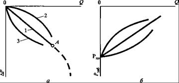
Based on the test data, Inflow Performance Relationship in the form of straight line (fig. 1) should be plotted. If the inflow performance relationship is curvilinear and convex to production rate axis, it means that filtration is nonlinear.

Fig. 1. Standard Inflow Performance Relationship:

а – in coordinates Q = f(∆P); б – in coordinates Q = f(Рbh)

The production rate convex inflow performance relationship (2 – fig. 1, а), are typical, as a rule, for depletion drives. It can be accounted for by various reasons:

–fracture closing if bottomhole pressure becomes lower than closure pressure; and

–reservoir oil degassing if bottomhole pressure becomes lower than bubble point pressure;

The production rate concave inflow performance relationship (3 – fig. 1, а), can be

obtained in the following cases:

–inflow increase under ∆Р increase caused by covering additional interlayers, fractures and so on;

–growing self-cleaning of bottomhole zone under underbalance and filtration resistance decline;

–new fraction formation;

–inaccurate test data (under actually unsteady-state flow). In such case it is necessary to repeat testing.

The linear inflow performance relationship is processed by Dupuis formula. The arbitrary points with coordinates Q′ and ∆Pпл′ should be taken on the straight line,

	and productivity factor КП =	Q′	is determined by them.
		∆P′
		пл
			94

Permeability factor can be calculated by Dupuis formula and productivity factor:

k =	КП ln rк	rc	(4)
	2πh

The nonlinear inflow performance relationship (curve 2 in fig. 1) can be processed

by two-term inflow formula. For this purpose, formula (1) should be put down as

follows:
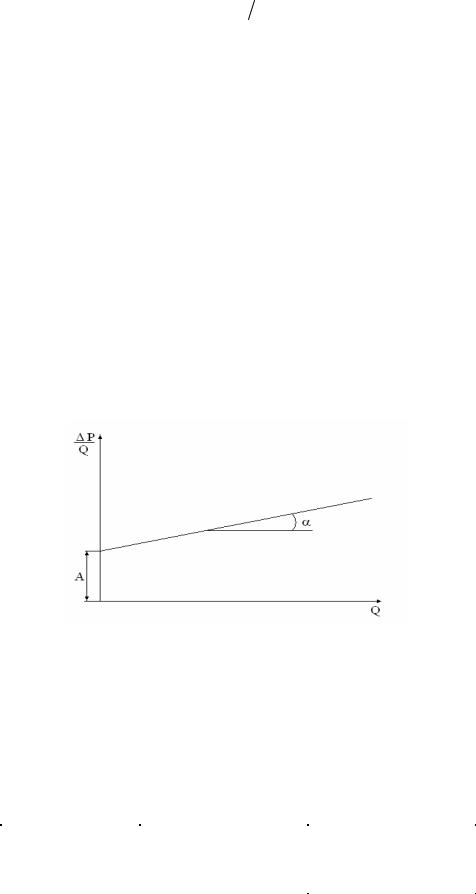
∆P = A + BQ		(5)
Q
	∆P
The inflow performance relationship is replotted in the coordinates		,Q
	Q

	(fig. 2).
	The straight line intercepts A in the axis of ordinates:
	A =		ln	rк		(6)
		2πkh		rc

The factor B = tgαis determined by inclination of line.

Fig. 2. Inflow Performance Relation Processing

by Two-Term Formula

Illustration of reservoir flow characteristics determination using well flow-after- flow test data

Given data:

Reservoir radius is 700 m, well radius is 10 cm, net oil thickness is 15 m and oil dynamic viscosity is 5 MPa·sec.

1 flow			2 flow			3 flow
Q,	∆Р,	Q,		∆Р,	Q,		∆Р,
m3/d	MPa	m3/d		MPa	m3/d		MPa
25	5	50		10	75		15
			95

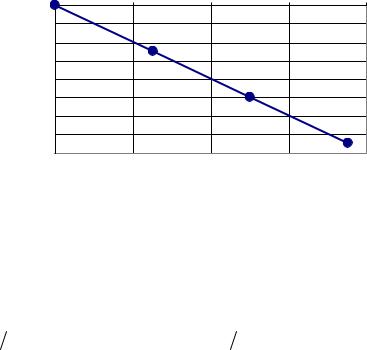
Inflow Performance Relationship:

Q, m3/d

	0	20	40	60	80
	0
	2
MPa	4
	6
Рbh,	8
	10
Рr-
	12
	14
	16

The inflow performance relationship is in the form of straight line coming out from the origin of coordinates, so, filtration is under liner filtration law.

Productivity factor:

КП =

Q

=

50

= 5

м3

= 5,8

10−11

м3

.

сут МПа

∆P 10

с Па

Permeability factor:

КП ln r

r

5,58 10−11 5 10−3 ln 700

0,1

−14

2

2

k =

к

c =

=

2,72 10

м

= 0,0272мкм

.

2 3,14 15

2πh

3. Pressure Build-up Measurement

Study of unsteady-state flow (unstable conditions of well operation) after well shutdown (or return of well to production) is aimed at obtaining data of mean integrated characteristics of formation zones. Any change of well operation processes is accompanied with pressure redistribution around it and such change depends on piezoconductivity of formation zones. The task of the study is to determine characteristics of bottomhole pressure change in the time function

Рbh=f(t) after changing well operation conditions (shutdown or brining to production).

Bottomhole pressure gage is lowered into the well operated under stable conditions (steady-state flow) with flow rate q. Then, well is shutdown and bottomhole pressure builds up to the value of formation pressure. The bottomhole pressure gage measures the bottomhole pressure build-up rate, and, based on the measurement data, the pressure build-up curve (fig. 3) is plotted.

Bottomhole pressure build-up of instantaneously shutdown imperfect oil well operated under stable production rate on homogeneous formation before shutting down can be expressed by the elastic drive equation:

96

P(t) = P	−	q	ln(	2.25χt	) .	(7)
		4πkh
0				r2
				пр

For convenience, this equation is put down in the form of the formula:

qµ

2, 25χt

qµ

2, 25χ

qµ

∆Рt

=

ln

=

ln

+

ln t ,

(8)

4πkh

2

4πkh

2

4πkh

rc

rc

or

∆Рt

= A + B ln t ,

(9)

where

В = tgα =

q

,

(10)

4πkh

А =

qµ

ln

2.25χ

,

(11)

4πkh

r2

пр

Р0 and Р(t) is bottomhole pressure before well shutdown and current bottomhole pressure (after shutdown); t is time after well shutdown; χ is piezoconductivity factor; and rПР is reduced well radius.

Fig. 3. Pressure Build-up Curve in Рt–t Coordinates

Formula (9) in the coordinates ∆Pt ,ln t is a straight line equation (fig. 4) with the slope of straight line В and intercept A. In actual practice, the form of pressure build-up curve is altered by still continuing fluid influx after well shutdown (noninstantaneous well shutdown), by changed bottomhole formation characteristics and others. As a rule, such factors alter the form of the initial portion of the curve and it should not be processed.

97

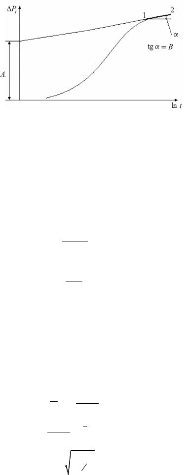
Fig. 4. Pressure Build-up Curve in ∆Pt , ln t Coordinates

The pressure build-up curve is processed as follows:

1.Pressure build-up curve is plotted in the coordinates Рt–t (fig. 3);

2.Pressure build-up curve is plotted in the coordinates ∆Pt −ln t (fig. 4);

3.Straight-line portion is singled out on the pressure build-up curve in the coordinates ∆Pt ,ln t ;

4.Slope of the singled out straight-line portion (slope В) is determined by the coordinates of the points corresponding to the origin and end of this portion:

В = y2 − y1 x2 − x1

5. Formation hydroconductivity is determined:

ε = q

4πB

6. Formation permeability is determined:

k = ε µ h

The reduced radius rпр is determined from the formula (6) by intercept А axis of ordinates, if piezoconductivity factor χ is known:

	А =	qµ	ln	2.25χ	= Вln	2.25χ	,
		4πkh		r 2		r 2
				пр		пр

ВА = ln 2.25χ,

rпр2

(12)

(13)

(14)

on Рt

2.25χ = еВА ,

rпр2

r	=	2.25χ	(м).	(11)
пр		еАВ
		98

The reduced radius rпр is compared with the well radius rс. The result of such comparison is C(S) factor which is termed Skin Factor:

rпр = rс e−C .			(12)
It follows thence:
С = ln	rc	.	(13)
	rпр

If С < 0, deliverability of the bottomhole zone is higher than that of the remote part of formation.

If С > 0, deliverability of the bottomhole zone is lower than that of the remote part of formation, and it is necessary to take measures for improving the deliverability of the bottomhole zone (bottomhole treatment).

If С = 0, it means that the bottomhole zone is not damaged by 1) formation drilling-in; 2) perforating and 3) development (perfect completion).

The skin factor can be also determined by Shchurov curve. In such case, piezoconductivity is determined by translating formula (11):

χ = 0, 44r 2	е	А	(13)
		В
пр

The value of skin factor is indicative of bottomhole treatment efficiency, for example, hydrochloric acid treatment. Decrease of the skin factor, for instance transition from the positive C value range to the negative C value range, or increase of negative skin factor in the absolute value is indicative of success of such treatment, i.e. improvement of deliverability (permeability) of the bottomhole zone.

The bottomhole treatment efficiency can be also judged by variability of reduced radius rпр. If rпр becomes higher, it means that deliverability of the bottomhole zone is improved and treatment is successful.

In addition to tangent method, pressure build-up curve can be also processed by other methods:

Horner Method is similar to tangent method. It considers well operation history before shutdown (duration of well operation with stable production rate before shutdown). Disadvantages of Horner methods are the same as those of tangent method.

Yu.P. Borisov Method is based on M. Masquete solution for point flow in infinite reservoir under time variable flow rate. The advantage of the method is low laboriousness, and disadvantage is low accuracy of calculating some derived quantities. R.I. Barenblatt and other Method is fairly laborious but such disadvantage is compensated by the main advantage of the method: approximate calculation of

99

integrals is much more accurate than approximate calculation of derived quantities of empirical function.

It is not easy to select a particular pressure build-up curve processing method. Most often, pressure build-up curve interpreter uses methods which are well known to him, or special software products.

Interpretation of pressure build-up curve data obtained by the above methods is given in table 1 (as illustration).

								Table 1
			Pressure Build-up Curve Processing Data
	Item				Permeability Factor, mcm2
		Well No.	Field	Tangent Method*				Barenblatt
	No.				Horner Method		Borisov Method
								Method
1		9	Aptugaiskoye	1.893	1.843		1.892	0.664
2		573	Sibirskoye	0.025	0.018		0.075	0.015
3		219	Shershnevskoye	1.235	1.256		1.331	0.152
4		307	Sibirskoye	0.053	0.036		0.031	0.032
5		501	Sibirskoye	0.182	0.181		0.087	0.166

Illustration of reservoir flow characteristics determination using data of well test under unsteady-state flows

Bottomhole pressure values for different time were obtained by production well test under unsteady-state flows after well shutdown (table 2). Oil with 1.5 MPa·sec flows in 10 m thick formation. Stable production rate before well shutdown was 50 m3/d.

Table 2

Item	t, с	Рt,	∆Pt,	ln t
No.		MPa	MPa
1	0	12.636	0
2	420	12.756	0.12	6.040255
3	720	12.925	0.289	6.579251
4	1020	13.074	0.438	6.927558
5	1320	13.223	0.587	7.185387
6	1620	13.371	0.735	7.390181
7	1920	13.519	0.883	7.56008
8	2220	13.667	1.031	7.705262
9	2520	13.816	1.18	7.832014
10	2820	13.934	1.298	7.944492
11	3420	14.151	1.515	8.137396
12	4020	14.299	1.663	8.299037
13	4620	14.388	1.752	8.43815
14	5220	14.467	1.831	8.560253
15	5820	14.516	1.88	8.669056
16	6420	14.556	1.92	8.767173
17	7020	14.566	1.93	8.856518
18	7620	14.596	1.96	8.938532
19	8820	14.616	1.98	9.084777
		100