Measurement and Control Basics 3rd Edition (complete book)

Chapter 1 – Introduction to Process Control

15

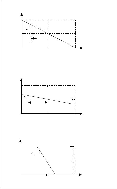
ratio. In Figure 1-12(b), where a low gain (Kc <1) is selected, a large change in error is required before the control valve would be fully opened or closed. Finally, Figure 1-12(c) shows the case of high gain (Kc >1), where a very small error would cause a large change in the control valve position.

The term proportional gain, or simply gain, arose as a result of the use of analytical methods in process control. Historically, the proportionality between error and valve action was called proportional band (PB). Proportional band is the expression that states the percentage of change in error that is required to move the valve full scale. Again, this had intuitive plausibility because it gave an operator a feel for how small of an error caused full corrective action. Thus, a 10 percent proportional band meant that a 10 percent error between SP and PV would cause the output to go full scale.

This definition can be related to proportional gain Kc by noting the following equation:

	PB =	1	x 100	(1-4)
		KC

An example will help you understand the relationship between proportional band and gain.

EXAMPLE 1-1

Problem: For a proportional process controller:

What proportional band corresponds to a gain of 0.4?

What gain corresponds to a PB of 400?

Solution:	a)	PB =		1		x 100 =	100		= 250%
				KC	0.4
	b)	KC =		1		x 100 =		100		= 0.25
				PB
					400

The modern way of considering proportional control is to think in terms of gain (Kc). The m term, as Equation 1-3 shows, has to be that control valve position that supplies just the right amount of hot water to make the temperature 100°F, that is, PV = SP. The position, m, indicated in Figures 1-12(a), (b), and (c), is often called the manual (m) reset because it is a manual controller adjustment.

16 Measurement and Control Basics

When a controller is designed to provide this mode of control, it must contain at least two adjustments: one for the Kc term and one for the m term. Control has become more complicated because it is now necessary to know where to set Kc and m for best control.

It would not take too long for the operator of our sample process to discover a serious problem with proportional control, namely, proportional control rarely ever keeps the process variable at the set point if there are frequent disturbances to the process. For example, suppose the flow to the tank suddenly increases. If the temperature of the tank is to be maintained at 100°F at this new rate of feed flow, more hot water must be supplied. This calls for a change in valve position. According to Equation 1-3, the only way that the valve position (V) can be changed is for the error (e) to change. Remember that m is a constant. Thus, an error will occur, and the temperature will drop below 100°F until an equilibrium is reached between the hot water flow and new feed flow. How much this drop will be depends on the value of Kc that was set in the controller as well as on the characteristics of the process. The larger Kc is, the smaller this offset will be in a given system.

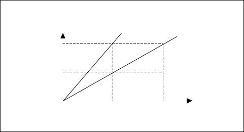
However, it can be shown that Kc cannot be increased indefinitely because the control loop will become unstable. So, some error is inevitable if the feed rate changes. These points are illustrated in Figure 1-13, which shows a plot of hot feed temperature versus hot water flow rate (valve position) for both low raw feed flow and high raw feed flow.

Hot Feed		Low Inlet	High Inlet
Temperature		Feed Flow	Feed Flow
T2
T1

Position 1

Position 2

Hot Water Valve Position

Figure 1-13. Sample process: Temperature vs. valve position

Chapter 1 – Introduction to Process Control

17

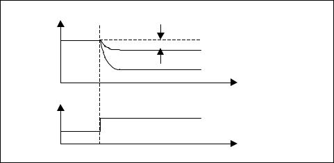
For the hot water valve in position 1 and the raw feed coming into the process tank at the low flow rate, the process would heat the fluid and produce hot feed fluid at temperature T2. If suddenly the feed went to the high flow rate and the valve position was not changed, the temperature would drop to T1. At this new high flow rate, the hot water valve must be moved to position 2 if the original temperature T2 is to be restored. Figure 1-14 shows the extent to which proportional control of the temperature valve can achieve this restoration.

Process Variable

	Offset	Set Point
		With proportional control
		No Control Action
		Time

Inlet Feed Flow

Step Change

Time

Figure 1-14. Process response with proportional control

One way to cope with the offset problem is by manually adjusting the m term. When we adjust the m term (usually through a knob on a process controller), we are moving the valve to a new position that allows PV to equal SP under the new conditions of load. In this case, with an increase in feed flow, Equation 1-3 clearly shows that the only way to obtain a new value for V, if e is to be zero, is by changing the m term. If process changes are frequent or large it may become necessary to adjust m frequently. It is apparent that some different type of control mode is needed.

Proportional-Plus-Integral Control

Suppose that the controller rather than the operator manually adjusts the proportional controller described in the previous section. This would eliminate the offset error caused by process changes. The question then is, on what basis should the manual reset be automated? One innovative concept would be to move the valve at some rate, as long as the error is not zero. Though eventually the correct control valve position would be found, there are many rates at which to move the valve. The most common practice in the instrumentation field is to design controllers that move the control valve at a speed or rate proportional to the error. This has

18 Measurement and Control Basics

some logic to it, in that it would seem plausible to move the valve faster as the error got larger. This added control mode is called reset or integral action. It is usually used in conjunction with proportional control because it eliminates the offset.

This proportional-plus-integral (PI) control is shown in Figure 1-15. Assume a step change in set point at some point in time, as shown in the figure. First, there is a sudden change in valve position equal to Kce due to the proportional control action. At the same time, the reset portion of the controller, sensing an error, begins to move the valve at a rate proportional to the error over time. Since the example in Figure 1-15 had a constant error, the correction rate was constant.

			Integral
Open			or Reset
				time
				ti			Reset Contribution
valve							KCe
							Proportional Contribution
position	KCe

Closed Time (t)

Error (e) + e

0 No error (SP = PV)

- e Time (t)

Figure 1-15. Proportional-plus-integral control

When time is used to express integral or reset action, it is called the reset time. Quite commonly, its reciprocal is used, in which case it is called reset rate in “repeats per minute.” This term refers to the number of times per minute that the reset action is repeating the valve change produced by proportional control alone. Process control systems personnel refer to reset time as the integral time and denote it as ti.

The improvement in control that is caused by adding the integral or reset function is illustrated in Figure 1-16. The same process change is used that was previously assumed under proportional-only control. Now, however,

Chapter 1 – Introduction to Process Control

19

Valve Position

V

Open

V

m

e error

Closed

0% SP

a) Gain of one, KC = 1

Valve Position

V

Open

V

e

Error

Closed

SP

0%

b) Low Gain, KC < 1.

Valve Position

V

Open

m

V

Closed

e

0%

SP

c) High Gain, KC > 1.

	Process Variable
100%	Range (0 to 100%)

Process Variable

Range (0 to 100%)

100%

Process Variable

Range (0 to 100%)

100%

Figure 1-16. Process response with PI control

20 Measurement and Control Basics

after the initial upset the reset action returns the error to zero and there is no offset.

Recognizing that the reset action moves the control valve at a rate proportional to error, this control mode is described mathematically as follows:

dV	= Ki e	(1-5)
dt

where

dV/dt = the derivative of the valve position with respect to time (t)

Ki	= an adjustable constant

We can find the position of the valve at any time by integrating this differential equation (Equation 1-5). If we integrate from time 0 to time, t, we obtain:

t
V = Ki ∫ edt	(1-6)
0

This equation shows that the control valve position is proportional to the integral of the error. This fact leads to the “integral control” label. Finally, combining proportional and integral control gives the total expression of a two-mode proportional-plus-integral (PI) controller:

t
V = Kce + Ki ∫ edt	(1-7)
0

If we let Ki = Kc/ti, we obtain an alternate form of the PI control equation in terms of the proportional constant, Kc, and the integral time, ti, as follows:

V = Kc e +	Kc		t	edt	(1-8)
			∫
	t	i
			0

One problem with PI control bears mentioning. If a control loop is using PI control, the possibility exists with the integral (reset) mode that the controller will continue to integrate and change the output even outside the operating range of the controller. This condition is called “reset windup.”

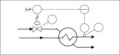
For example, the heat exchanger shown in Figure 1-17 can be designed and built to heat 50 gal/min of process fluid from 70°F to 140°F. If the process flow should suddenly increase to 100 gal/min, it may be impossible to supply sufficient steam to maintain the process fluid temperature at 140°F even when the control valve is wide open (100%), as shown in Fig-

Chapter 1 – Introduction to Process Control

21

IA	TY	TIC
	200	200
	I/P
	TV
	200
Steam		TT	TE
		200	200
Process			Process
Fluid			Fluid
	E-200		Condensate
Figure 1-17. Heat exchanger temperature control

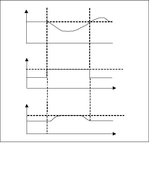
ure 1-18. In this case, the reset mode, having opened the valve all the way (the controller output is perhaps 15 psig), would continue to integrate the error signal and increase the controller output all the way in order to supply pressure from the pneumatic system. Once past 15 psig, the valve will open no further, and the continued integration serves no purpose. The controller has “wound up” to a maximum output value.

Further, if the process flow should then drop to 50 gal/min (back to the operable range of the process), there would be a period of time during which the controlled temperature is above the set point while the valve remains wide open. It takes some time for the integral mode to integrate (reset) downward from this wound-up condition to 15 psig before the valve begins to close and control the process.

It is possible to prevent this problem of controller-reset windup by using a controller operational feature that limits the integration and the controller output. This feature is normally called anti-reset windup and is recommended for processes that may periodically operate outside their capacity.

Proportional-Plus-Derivative (PD) Control

We can now add to proportional control another control action called derivative action. This control function produces a corrective action that is proportional to the rate of change of error. Note that this additional correction exists only while the error is changing; it disappears when the error stops changing, even though there may still be a large error.

22 Measurement and Control Basics

Temperature
SP	(1400F)

Time (t)

Inlet Feed

Flow (GPM)

	100	Step Change
	50
		Time (t)
	Controller
	Output (%)
	100	windup
	75
		Time (t)
	Figure 1-18. Reset windup control

Derivative control can be expressed mathematically as follows:

	V = Kd	de	(1-9)
		dt

where

Kd	= the derivative constant

de/dt = the derivative of the control system error with respect to time

The derivative constant Kd can be related to the proportional constant Kc by the following equation:

Kd = Kctd

(1-10)

Chapter 1 – Introduction to Process Control

23

where td is the derivative control constant. If we add derivative control to proportional control, we obtain

	V = Kc e + Kctd	de	(1-11)
		dt

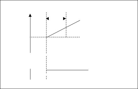
To illustrate the effects of PD control, let's assume that the error is changing at a constant rate. This can be obtained by changing the set point at a constant rate (i.e., SP = ct), as shown in Figure 1-19.

Valve

Position

Proportional

Contribution

Derivative

Contribution

td

Time(t)

Set Point

e = ct

Time(t)

Figure 1-19. Proportional-plus-derivative

Derivative action contributes an immediate valve change that is proportional to the rate of change of the error. In Figure 1-19, it is equal to the slope of the set point line. As the error increases, the proportional action contributes additional control valve movement. Later, the contribution of the proportional action will have equaled the initial contribution of the rate action. The time it takes for this to happen is called the derivative time, td. The ramped error can be expressed mathematically as follows:

e = Ct

(1-12)

24 Measurement and Control Basics

where
e	= the control loop error
C	=	a constant (slope of set point change)
t	=	time

If we substitute this value (e = Ct) for the control loop error into the equation for a PD controller, we obtain

	V = KcCt + Kctd	d (Ct)	(1-13)
		dt

Since the derivative of Ct with respect to time, t, is simply equal to C, the control action (V) from the PD controller to the control valve becomes

V = KcC(t + td )

(1-14)

This indicates that the valve position is ahead in time by the amount td from the value that straight proportional control would have established for the same error. The control action leads to improved control in many applications, particularly in temperature control loops where the rate of change of the error is very important. In temperature loops, large time delays generally occur between the application of corrective action and the process response; therefore, derivative action is required to control steep temperature changes.

Proportional-Integral-Derivative Control

Finally, the three control functions—proportional, integral, and derivative —can be combined to obtain full three-mode or PID control:

	K		t	de	(1-15)
V = Kc e +		c	∫ edt + Kctd
	t			dt
	i		0

Deciding which control action (i.e., PD, PID, etc.) should be used in a control system will depend on the characteristics of the process being controlled. Three-mode control (PID) cannot be used on a noisy measurement process or on one that experiences stepwise changes because the derivative contribution is based on the measurement of rate of change. The derivative of a true step change is infinite, and the derivatives of a noisy measurement signal will be very large and lead to unstable control.

The PID controller is used on processes that respond slowly and have long periods. Temperature control is a common example of PID control because the heat rate may have to change rapidly when the temperature measure-