Encyclopedia of Sociology Vol

TIME SERIES ANALYSIS

ters. However, this is an aesthetic yardstick that may have nothing to with the substantive story of interest.

USES OF ARIMA MODELS IN SOCIOLOGY

It should be clear that ARIMA models are not especially rich from a substantive point of view. They are essentially univariate descriptive devices that do not lend themselves readily to sociological problems. However, ARIMA models rarely are used merely as descriptive devices (see, however, Gottman 1981). In other social science disciplines, especially economics, ARIMA models often are used for forecasting (Granger and Newbold 1986). Klepinger and Weiss (1985) provide a rare sociological example.

More relevant for sociology is the fact that ARIMA models sometimes are used to remove ‘‘nuisance’’ temporal dependence that may be obstructing the proper study of ‘‘important’’ temporal dependence. In the simplest case, ARIMA models can be appended to regression models to adjust for serially correlated residuals ( Judge et al. 1985, chap. 8). In other words, the regression model captures the nonstationary substantive story of interest, and the time series model is used to ‘‘mop up.’’ Probably more interesting is the extension of ARIMA models to include one or more binary explanatory variables or one or more additional time series. Nonstationarity is now built into the time series model rather than differenced away.

Intervention Analysis. When the goal is to explore how a time series changes after the occurrence of a discrete event, the research design is called an interrupted time series (Cook and Campbell 1979). The relevant statistical procedures are called ‘‘intervention analysis’’ (Box and Tiao 1975). Basically, one adds a discrete ‘‘transfer function’’ to the ARIMA model to capture how the discrete event (or events) affects the time series. Transfer functions take the general form shown in equation (1):

(1 − δ1B− −δ1Br)yt=(ω0−ω1B− −ωsBs)xt−b.

If both sides of equation (1) are divided by the left-hand side polynomial, the ratio of the two polynomials in B on the right-hand side is called a transfer function. In the form shown in equation (1), r is the order of the polynomial for the ‘‘dependent variable’’ (yt), s is the order of the polyno-

mial for the discrete ‘‘independent variable’’ (xt), and b is the lag between when the independent ‘‘switches’’ from 0 to 1 and when its impact is observed. For example, if r equals 1, s equals 0, and b equals 0, the transfer function becomes ω0/1-δ1. Transfer functions can represent a large number of effects, depending on the orders of the two polynomials and on whether the discrete event is coded as an impulse or a step. (In the impulse form, the independent variable is coded over time as 0,0, . . . 0,1,0,0, . . . ,0. In the step form, the independent variable is coded over time as 0,0, . . .

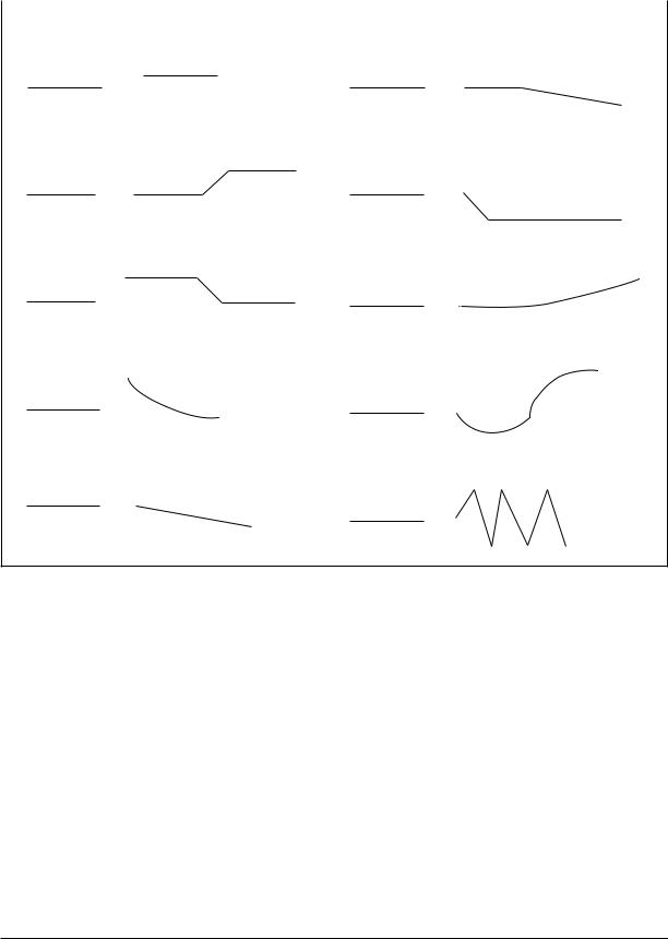
1,1 . . . 1. The zeros represent the absence of the intervention, while the ones represent the presence of the intervention. That is, there is a switch from 0 to 1 when the intervention is turned on and a switch from 1 to 0 when the intervention is turned off.) A selection of effects represented by transfer functions is shown in Figure 6.

In practice, one may proceed by using the time series data before the intervention to determine the model specification for the ARIMA component, much as was discussed above. The specification for the transfer function in the discrete case is more ad hoc. Theory certainly helps, but one approach is to regress the time series on the binary intervention variable at a moderate number of lags (e.g., simultaneously for lags of 0 periods to 10 periods). The regression coefficients associated with each of the lagged values of the intervention will roughly trace out the shape of the time path of the response. From this, a very small number of plausible transfer functions can be selected for testing.

In a sociological example, Loftin et al. (1983) estimated the impact of Michigan’s Felony Firearm Statute on violent crime. The law imposed a two-year mandatory add-on sentence for defendants convicted of possession of a firearm during the commission of a felony. Several different crime time series (e.g., the number of homicides per month) were explored under the hypothesis that the crime rates for offenses involving guns would drop after the law was implemented. ARIMA models were employed, coupled with a variety of transfer functions. Overall, the intervention apparently had no impact.

3151

	TIME SERIES ANALYSIS
Abrupt change in level	Delayed change in direction
(I)	(I)
Delayed change in level	Temporary change in direction
(I)	(I)

Temporary change in level

Accelerated change in direction

(I)

(I)

Decaying change in level

"Evolutionary operations" effect

(I)

Change in variability

Abrupt change in direction

(I)	(I)

Figure 6. A Sampler of Intervention Effects. I = Intervention

Multiple Time Series. ARIMA models also may be extended to more than one time series (Chatfield 1996, Chap. 10) Just as the goal for the univariate case was to find a model that transformed the single time series into white noise, the goal for the multivariate case is to find a model that will transform a vector of time series into a white noise vector. In effect, each series is regressed simultaneously not only on lagged functions of itself and the disturbance term but on functions of all other time series and their disturbance terms. In practice, this sometimes reduces to building transfer function models that include a single response time series and several input time series, much as in multiple regression. For exam-

ple, Berk et al. (1980) explored how water consumption varied over time with the marginal price of water, weather, and a number of water conservation programs.

The mathematical generalization from the univariate case is rather straightforward. The generalization of model specification techniques and estimation procedures is not. Moreover, multivariate time series models have not made significant inroads into sociological work and therefore are beyond the scope of this chapter. Interested readers should consult Chatfield (1996) for an introduction or Granger and Newbold’s (1986) for a more advanced treatment.

3152

TIME USE RESEARCH

CONCLUSIONS

Time series analysis is an active enterprise in economics, statistics, and operations research. Examples of technical developments and applications can be found routinely in a large number of journals (e.g., Journal of the American Statistical Association, Journal of Business and Economic Statistics, Journal of Forecasting). However, time series analysis has not been especially visible in sociology. Part of the explanation is the relative scarcity of true time series for sociological variables collected over a sufficiently long period. Another part is that time series analysis is unabashedly inductive, often making little use of substantive theory; time series analysis may look to some a lot like ‘‘mindless empiricism.’’ However, in many sociological fields, true time series data are becoming increasingly available. Under the banner of ‘‘data analysis’’ and ‘‘exploratory research,’’ induction is becoming more legitimate. Time series analysis may well have a future in sociology.

(SEE ALSO: Longitudinal Research; Statistical Methods)

Freedman, D. A., and David Lane 1983 ‘‘Significance Testing in a Nonstochastic Setting.’’ In P. J. Bickel, K. A. Doksum, and J. L. Hodges, Jr., eds., A Festschrift for Erich L. Lehman. Belmont, Calif.: Wadsworth International Group.

Goldberg, Samuel 1958 Introduction to Difference Equations. New York: Wiley.

Gottman, J. M. 1981 Time-Series Analysis. Cambridge, UK: Cambridge University Press.

Granger, C. W. J., and P. Newbold 1986 Forecasting Economic Time Series. Orlando, Fla.: Academic Press.

Harvey, A. C. 1990 The Econometric Analysis of Time Series, 2nd ed. London: Harvester Wheatshear.

Hsiao, Cheng 1986 Analysis of Panel Data. Cambridge, UK: Cambridge University Press.

Judge, D. G., W. E. Griffiths, R. C. Hill, H. Lutkepohl, and T.-C. Lee 1985 The Theory and Practice of Econometrics. New York: Wiley.

Kessler, D. A., and S. Duncan 1966 ‘‘The Impact of Community Policing in Four Houston Neighborhoods.’’ Evaluation Review 6(20):627–669.

Klepinger, J. D. H., and J. G. Weis 1985 ‘‘Projecting Crime Rates: An Age, Period, and Cohort Model Using ARIMA Techniques.’’ Journal of Quantitative Criminology 1:387–416.

REFERENCES

Berk R. A. 1988 ‘‘Causal Inference for Sociological Data.’’ In N. Smelser, ed., The Handbook of Sociology. Newbury Park, Calif.: Sage.

———, T. F. Cooley, C. J. LaCivita, S. Parker, K. Sredl, and M. Brewer 1980 ‘‘Reducing Consumption in Periods of Acute Scarcity: The Case of Water.’’ Social Science Research 9:99–120.

Box, G. E. P., and G. M. Jenkins 1976 Time Series Analysis: Forecasting and Control. San Francisco: Holden-Day.

———, and G. C. Tiao 1975 ‘‘Intervention Analysis with Applications to Economic and Environmental Problems.’’ Journal of the American Statistical Association

70:70–79.

Chamlin, Mitchel B. 1988 ‘‘Crime and Arrests: An Autoregressive Integrated Moving Average (ARIMA) Approach.’’ Journal of Quantitative Criminology

4(3):247–258.

Chatfield, C. 1996 The Analysis of Time Series: An Introduction, 5th ed. New York: Chapman and Hall.

Cook, T. D., and D. T. Campbell 1979 Quasiexperimentation. Chicago: Rand McNally.

Cox, D. R., and D. Oakes 1984 Analysis of Survival Data: London: Chapman and Hall.

Loftin, C., M. Heumann, and D. McDowall 1983 ‘‘Mandatory Sentencing and Firearms Violence: Evaluating an Alternative to Gun Control.’’ Law and Society Review 17(2):287–318.

———, and D. McDowall 1982 ‘‘The Police, Crime, and Economic Theory.’’ American Sociological Review

47:393–401.

RICHARD A. BERK

TIME USE RESEARCH

Time provides the organizational key to action at the level of individuals, groups, and institutions. It also defines a normative framework that regulates interpersonal relationships and allows synchronized operations in different parts of society. In the concept of time, structural as well as symbolic facets assume significance. In fact, as it is conceived in sociological theory, time is a means of social coordination as well as a dimension that assigns value to action schemes in a system assuring social order (Pronovost 1989; Sue 1994).

The empirical study of the temporal organization of human action reveals the functional charac-

3153

TIME USE RESEARCH

teristics of social roles and the societal division of social tasks. For instance, indicators of inequality and social exclusion can be derived and compared by referring to estimates of the amount of time involved in gender-related activities such as market work and housework. The time use of populations or subpopulations is studied mostly by means of diary procedures that assess individual ‘‘time budgets:’’ the sequence, timing, and duration of activities performed by individuals over a specified period. It is misleading to think that the aim of time budget research is time as either a physical or a subjectively perceived entity. As stressed by the major postwar promotor of this area of study, the Hungarian sociologist Szalai, the object of studying time is to discover the use people make of their time, or ‘‘the arrangement and the fit of people’s activities in a temporal frame of reference, the temporal order and structure of everyday life’’ (1984, p. 20).

From this point of view, time is a special kind of resource. As with material goods and more symbolic commodities such as money, people have a ‘‘fund’’ of time at their disposition and make decisions on how to use, ‘‘spend,’’ or ‘‘invest’’ it. However, time is a far more democratic resource in that every person deals with the same basic ‘‘stock’’ of it, such as the twenty hours in a day and the seven days in a week. This means that a shared reference of differential time allocation patterns can facilitate coherent comparisons and meaningful interpretations. It is this particular aspect that has made time use an important topic in quantitative social research. Both academic scholars and national statistical offices have shown a growing interest in time-budget data because those data permit policy-oriented microanalyses of changing lifestyles at the individual or household level as well as macroanalyses of social and economic inequalities in the context of cross-national comparative studies.

In contrast to the physical notion that attributes equivalent temporal resources to all people and therefore facilitates systematic accounts, from a subjective point of view, the length of a day is not always the same. Some people seem to have more time than others. This phenomenon reveals the sociopsychological dimension of time in which concepts such as stress and alienation are relevant. In a world where the quality of life depends largely

on what one gets out of the time at one’s disposal, coping with time and compressing multiple activities into the same time slot have become important skills. Furthermore, it is a universal observation that boring periods during a day, week, or year can seem long, whereas other, quantitatively equivalent but exciting periods of time are perceived as a passing moment. However, in studying social time, time-budget research adopts an activi- ty-oriented approach and focuses only indirectly on subjective experiences. In substance, this means that observable patterns of behavior are selected as primary evidence and, in methodological terms, standard time units are chosen for measurement purposes.

THE TIME USE RESEARCH TRADITION

Although social time is not intrinsically quantitative, the use of standard time units for the purposes of analyzing the structure of everyday life seems legitimate, since the transfer of human work from agriculture to artificially controlled industrial environments and the subsequent changes in civilization have largely transformed natural time (tied to seasonal conditions and biological needs) into conventional, rational time (Elias 1988). As a corollary to this process, social life has become dominated by timekeeping. This chronometric function is characterized by a universally accepted ‘‘time’’ language that coordinates rhythms of action in the public and private spheres (Zerubavel 1982). Therefore, time budgets, which are concerned with different kinds of schedules for structuring the flow of events, are a key to the systematic investigation of the complex interdependencies and trade-offs of modern life.

The historical origins of the study of social time lie in both sociological theory and empirical research. With regard to theory, the early French school of sociology was interested in this phenomenon from the point of view of the historical and anthropological dimensions of social change (Pronovost 1989). Around the turn of the century, Hubert, Mauss, Durkheim, and Halbwachs conceived of social time as an intrinsically qualitative phenomenon that was relevant for the characterization of the sacred-profane symbolic dichotomy in the evolution of the collective consciousness or

3154

TIME USE RESEARCH

the formation of a collective memory. Their focus was a macro one, and their main interest was to explain long-term cultural change.

In contrast, Mead in the early 1930s chose an individualistic, micro-oriented approach that offered a philosophical rationale for studying time in the present. The present was conceived of as the context for the emergence and assimilation of various social time systems in interplay with the definition of different notions of ‘‘the self.’’ Thus, the French and American approaches represent polar opposites, with one conceiving time within the matrix of historical societal relationships, and the other from the perspective of mutable configurations of symbolic interactions in small groups. The somewhat later work of Sorokin reflects both approaches. He presents the functionalist idea that the plurality of individual time schemes requires extensive synchronization to achieve social cohesion and that time expresses the sociocultural ‘‘pulsation’’ of a society.

In the 1960s, Gurvitch gave new impetus to the study of time after a considerable period of neglect. He was the first to conceive of time as an important source of contradictions and potential conflict. In particular, he stressed the hierarchically diversified aspects of the phenomenon (e.g., social time, time in organizations, time in special social groups) and raised the issues of power and legitimacy. More recently, Merton introduced the concept of ‘‘socially expected durations’’ that highlight the normative aspects of the embeddedness of time in social structures. In contrast, Elias stressed the role of time as a symbolic means of social regulation but also of increasingly unpredictable individual self-expression.

The historical origins of empirical investigations of social time are even older, going back to the middle of the nineteenth century. Three lines of research are significant: the research conducted by Friedrich Engels on the English working class, where the temporal organization of daily life was the issue; the studies undertaken by Frédéric LePlay, in which the economic ‘‘family-budgets’’ of workers in several European countries were assessed (similar to what ‘‘time budgets’’ do today); and the experimental work on time and motion performed by Frederick Taylor, based on carefully collected chronometric data. Taylor’s aim was to introduce

strategies of scientific time management in industry. In regard to the adoption of time-budget methodologies, there were Bevans’s pioneering studies (1913) of how workers spent their spare time and early Soviet inquiries by Strumilin into time use as the basis for rational social programming. Lundberg and Komarovsky’s research into the organization of time within the realm of community research was conducted along the lines of American cultural anthropology.

Of more enduring interest, however, were two studies published in the 1930s. Jahoda et al.’s

Marienthal: The Sociography of an Unemployed Community (1933) was a substantial contribution to the study of time use. It explores changes in the meaning of time for German working-class families when work, as a dominant regulating and legitimizing criterion for time use, has disappeared. Male workers tended to become severely disoriented and alienated after losing their work-based prestige, whereas their wives were successful in mastering that situation because they had much more positive attitudes based on more complex sources of social recognition. This research also shows how important it is to be aware that similar circumstances can assume diverse meanings for different groups.

The other study, whose importance lies in its methodological ideas, is Sorokin and Berger’s TimeBudgets and Human Behavior (1939). Here the aim was to explore meaningful criteria for decision making conducive to different time structures. Information on motivations and the kinds of experiences associated with certain practices and future projects was collected to acquire a deeper understanding of how people deal with their time. Even more important, this research raised the crucial epistemological question of how to divide essentially continuous strings of behavior into activity segments that, beyond commonsense classifications, can be grouped into homogeneous and mutually exclusive categories (Kurtz 1984). The difficulty was that some activities that from an external viewpoint seemed identical could assume unequal functions in the eyes of those concerned, or conversely, that substantially different activities could assume similar functions. This means that any classification of activities presupposes an interpretive act. With this fundamental problem

3155

TIME USE RESEARCH

in mind, these authors were forced to approach earlier and purely descriptive assessments of time allocation with skepticism and spell out the methodological issues in their research.

After World War II, research took different directions in accordance with divergent political ideologies. The assessment of living conditions, which involved obtaining background data for economic planning and monitoring centrally initiated social change, continued to be of pivotal importance in research in eastern Europe’s communist countries. Prudensky’s time-budget studies in the Soviet Union in the 1960s not only followed the direction of Strumilin’s work but also reflected these ideological concerns. The need to broaden data gathering to obtain effective guidance for public policy at the national level led Hungary’s statistical office to begin the first microcensus research in this field.

In capitalist societies, time use research was concerned principally with mass media and leisure culture. Pioneering time use studies of audiences were undertaken by the BBC as well as NHK, the Japanese radio and television system, using largescale survey techniques. From 1960 onward, NHK conducted regular five-year follow-up rounds of research to obtain time series statistics that showed long-term longitudinal development. This was a useful strategy because it produced an interesting account of how, in terms of time use, traditional ways of life are supplanted by innovative, primarily television-centered styles.

This was the situation in 1963, when the idea of conducting a Multinational Comparative Time Budget Research Project emerged. This was an ambitious sociological initiative in light of the organizational and data-processing difficulties of those years. Launched by a group of scholars directed by Szalai, sponsored by UNESCO’s International Social Science Council, and coordinated by the Vienna Centre, this project attempted to obtain an interculturally valid body of knowledge that would shed light on regularities or variations in the functioning of human societies with regard to time use. This information was to be derived from a database of twelve different countries by using methodological instruments that assured a high level of analytic precision (Szalai 1977). In organizing the initiative, the basic concern was to

avoid the emergence of a single central vantage point regarding the collection, elaboration, and interpretation of information. Therefore, research sites had considerable autonomy in studying the uniform data sets collected by means of strictly standardized survey instruments from probability samples of urban populations in the twelve countries under investigation.

From a positivist point of view, the focus on chronometric evidence and on an array of ‘‘hard’’ time use indicators enhanced the scientific character of the study and facilitated the collaboration of teams from such culturally and sociopolitically different environments as the United States and the Soviet Union. Of course, collaboration entailed the acceptance of common working hypotheses such as the expected influence of the major independent variables of industrialization and urbanization on the modalities of the division of market work and nonmarket work in households. By contrast, time for leisure was thought to be correlated with superior levels of modernization and democratization. These hypotheses clearly reflected the research traditions of the day, and so to connect the ideologically distant worlds of the 1960s, it was necessary to choose highly conventionalized and neutral time indicators as empirical evidence.

The Twelve Country Project, characterized by a strong belief in the ‘‘scientific and social import of cross-national comparative research’’ (Szalai 1977), did not go without criticism. Some thought that it was most important for cross-national research to contribute findings on general theoretical problems (Przeworski and Teune 1970). However the promoters were convinced that the discovery of the empirical peculiarities of cultural settings was at least as important as the verification of a priori hypotheses on common characteristics and trends. That the pragmatic point of view prevailed meant that the problem of a lack of reliable, relevant, and usable data had to be overcome.

In retrospect, it seems that this project did not contribute much to general theory, but it did produce an elaborate methodology whose essential lines are applied to basic and official survey research in many countries today. In fact, as Szalai hoped, the homogenization of time-budget methods now permits the drawing of ‘‘maps’’ of collec-

3156

TIME USE RESEARCH

tive daily activity schemes at different levels of definition that have proved to be useful diagnostic elements for many policymakers and grassroots organizations. When economic indicators are insufficient, statistical information regarding the use of time can open up new policy perspectives and guide substantial change, especially when gaps in the quality of life manifest themselves and corrective action is needed to improve the conditions of disadvantaged social groups.

METHODOLOGICAL ASPECTS OF TIME-

BUDGET RESEARCH

Since the work of Szalai, the methodology of time use research has been further refined. Under the auspices of the International Association of Time Use Research, in particular under the guidance of Harvey (1984, 1993), who has repeatedly codified the best practices, statistical bodies have reached a consensus on the format of official survey research.

The task of discovering the temporal order and structure of everyday life by means of timebudget methods involves fax more complex activities than gathering simple answers to questions of who does what, when, where, and with whom. In the design of a time-budget study, methodological issues such as the scope and scale of the research, the population from which the sample is to be drawn, the format of the data-gathering instruments, the classification and coding of activities, the choice of basic indicators, and the validity and reliability of the data must be resolved.

Defining the scope of a study also means fixing its scale. In fact, a time use survey may deal with a special group of persons, such as working women or teenagers, or with comprehensive national populations, perhaps excluding preschoolers. Or it may focus on a daily activity such as housework and child care or leisure. Alternatively, it may attribute equal weight to all everyday pursuits. Finally, the study may be aimed at discovering how the time of a special kind of day is spent, may take into account the rhythm of the week by distinguishing workdays from Sundays, or may be interested in longer periods such as the year with its seasonal differences and, in the extreme case, the life cycle (which of course would have to be studied on the basis of long-term recollections). Theo-

retically grounded sociological research is, for economic reasons, more likely to have circumscribed objectives, whereas national statistical offices have all-encompassing multipurpose datasets available. However, in both cases, the predominant tendency is to focus on the twenty-four hours of one or more single days in the life of the respondent. When these days are distributed over the week, month, or year, the average profiles of the period can be synthetically reconstructed. Such profiles most often refer to uninterrupted sequences of nonoverlapping main or ‘‘primary’’ activities. When there is interest in ‘‘secondary’’ activities or, more precisely, in contemporaneous activity episodes, the respondent usually is asked to designate the elements that represent the principal flow, which typically covers the 1,440-minute arc of the day. In fact, leaving secondary activity out of focus furnishes an unduly simplified picture of what is going on, since it ignores efficiency strategies that enable people who are short of time to deal simultaneously with multiple jobs. This frequently criticized weakness is compensated for by the heuristically valid fact that strict 24-hour accounts produce agile descriptive models. With such models, whatever time is saved on one kind of activity is strictly accredited, using zero-sum logic, to one or more other activities. Therefore ‘‘time set free’’ and the equivalent ‘‘time gained’’ concept furnish concise indicators of social change. Tracing the balance of the two magnitudes gives a dynamic slant to the analysis of time use and sheds light on the spectrum of strategic options.

Depending on the scope of the study, populations and samples are variously defined. From this point of view, the most significant difference between time use studies regards the choice of the sampling unit, which may be the individual or the household. In earlier studies, individual time use was of primary concern, and so estimates were obtained by classifying persons by their sociodemographic characteristics. More recent research, however, has looked more into how different types of families, as molecular units, manage time allocation with regard to income generation as well as work in the sphere of home and child care. Statistical offices now use very large probability samples of households to be able to generate cross-tabulated data on specific territorial areas and particular social groups. In Italy, for instance,

3157

TIME USE RESEARCH

the last national time use survey, conducted by Istat in 1988 and 1989, consisted of more than 38,000 persons belonging to almost 14,000 households. A survey conducted in Germany in 1991 and 1992 by the Statistisches Bundesamt included 7,200 households. One of the most difficult problems in time-budget research is the sample units’ frequent refusal to respond once they see how much time is involved. In fact, nonresponse rates tend to be high and in some official surveys amount to almost 30 percent. This problem is easier to handle in smaller-scale studies, which often use quota sampling.

Data gathering in time use research begins with an interview (Scheuch 1972) to record the characteristics of the respondent and his or her family, contractual work arrangements, normal labor supply, and housing or other assets and to inquire into irregularities in the day designated for collecting the time-budget information. The time budget itself is registered in a protocol, a diary, or modular display where the beginning and the end of each activity can be indicated together with other information. The resulting datasets show for each day and respondent (1) the number of different activities performed and the frequency of each activity in separate episodes (for instance, the series of daily meals or the periods passed in front of the television set) and (2) the timing, duration, and sequence of activities or activity episodes. Most often, the interviewees register activities by using their own words. A grid of minimal time intervals is given (the ‘‘fixed interval’’ solution), where the task is to fill each interval with an activity, or the interviewee is asked to specify the exact time points of his or her schedule (the ‘‘open interval’’ solution). To obtain the essential elements of the interviewee’s context, there is usually room to indicate contemporaneous activities (for instance, reading while using public transport or listening to music while doing homework); participation in activities with family members, neighbors, friends, and colleagues; and where the activity takes place. The least expensive method of data collection is the condensed telephone interview, which explores time use on the previous day. For field studies, there are other procedures, such as single face-to-face interviews and two personal interviews. In the first case, the person is asked to recall what he or she did the preceding day. This

procedure is complicated when a lot of detail is required. The second procedure involves two personal interviews. During the first, background information is collected and the time use diary is left behind, to be filled in the next day. During the second interview, on the day after the respondent’s observation of his or her time use, the interviewer checks and refines the registrations. In Scandinavian countries, people were asked to return diaries by mail. This saves a second visit, but it is advisable only when intelligent and conscientious collaboration can be assumed.

The greatest methodological challenge in time use research is the choice of the scheme of classification of activities in terms of which the structure of everyday life is represented. Sorokin started to tackle this problem, but convincing theoretical or empirical criteria for constructing typological keys have not been found, and using conventional categories of ordinary language is not entirely satisfactory. Normative and/or contractual work arrangements suggest a fairly unambiguous specification of ‘‘market work,’’ but there are some activities in the home that, according to circumstances, can be classified as either housework or leisure. This difficulty could be overcome if the respondent did the coding himself or herself, but usually the log of daily routines is described in the respondent’s own words and codification is done by someone else, following criteria that exclude personal and/or subjective meanings. An even more fundamental issue is whether current classifications can be assumed to be meaningful in cross-cultural terms. Time use studies distinguish the minimal basic activity groupings of personal needs, formal work or education, household work, and leisure. The hidden dimension that is postulated by such groupings is obviously a reflection of the Western opposition between necessity and freedom of choice. It places market work immediately after biological needs and before domestic work, which is placed near leisure. This implicitly individualistic and work-oriented, contractual rationale probably is not well suited to representing the more solidarityoriented temporal orders of everyday life in traditional societies (Bourdieu 1963).

Another difficulty concerns the level of specificity at which a common array of activities is reported at the collective level. The daily pursuits

3158

TIME USE RESEARCH

of persons who lead a busy life can be meaningfully recorded in great detail, whereas those of persons tied to the home usually have much less texture. One way to approach this difficulty is to construct hierarchical coding frameworks in which the first column in a multiple-digit code divides the day in terms of major classes of activities. Additional columns focus on increasingly more complex but exhaustive time accounts. The time use project coordinated by Szalai identified in its timebudget protocols ninety-six activity categories. For some purposes, these were reduced to thirty-seven and, for others, to the following ten main groups: work, housework, child care, shopping, personal needs, education, organizational activity, entertainment, active leisure, and passive leisure. Today the coding schemes for official statistical surveys often include many more basic activity categories because they have to accommodate the heterogeneity of lifestyles across gender groupings, generations, occupational categories, and rural versus urban residential environments.

Once time-budget data have been collected and coded, decisions about data processing and indicator construction can be made. According to the complexity of statistical data elaborations, there are three different levels of analysis (Stone 1972, pp. 96–97). First, activity arrays in terms of frequencies or durations, possibly taking company or locations into account, are cross-tabulated with the sociodemographic characteristics of the actors. Second, single activities and their positioning during the course of the day are studied. Finally, stochastic activity sequences are analyzed, focusing on the structure and rhythm of chronological daily routines. Since the 1960s, the following set of indicators generally have been used in computations: (1) the generic average duration of an activity, where the numerator refers to the total sample, disregarding whether there was involvement in the activity, (2) the rate of participation, or the percentage of interviewees who were involved in an activity, and (3) the specific average duration of an activity, where the denominator includes only those who have engaged in it.

Another issue in these surveys is the validity and reliability of data sets. Questions of validity can be raised by difficulties in recall and incorrect identification of activities among respondents or

by possible alterations of spontaneous behavior after observation and the consequent distortions in reports or by research instruments that inadequately reflect the specificities of the observed sociocultural context. Research directed at data quality ( Juster 1985; Niemi 1993) has shown that results obtained by means of time budgets present at the aggregate level a high correlation with those obtained by means of other forms of observation, such as interviews, workplace or school statistics, and telephone surveys. Moreover, the hypothesis that the desirability or social prestige of certain activities or lifestyles could influence time use reports has not been confirmed. In general, it seems that the twenty-four-hour frame of reference helps reduce such effects and brings informal and often undeclared work commitments to light. Certainly, activities that are assumed to be of secondary importance, such as conversations and listening to the radio, are under represented in current summary tables that restrict the attention to ‘‘primary’’ time allocations. However, this cannot be considered an invalidating shortcoming. Nevertheless, to assure validity, time budgets presuppose the concept of rational time. If a population does not live by the clock, any calculation of time budgets is meaningless.

CONTRIBUTIONS OF TIME USE

RESEARCH

Time use research has gained momentum because of interest on the part of international agencies in comparing the functioning of societies in their national settings, the need to connect demographic change and social development, the need to focus on gender-related or generational variables to understand the changing role of the family, the awareness that economic variables reflect wealth and well-being only in very partial ways and that household and care activities must be brought into focus, and the need to construct articulated databases for decision making about social policy.

Since the late 1980s, nationally representative time use data sets have been available for several countries, but the evidence is not easy to compare because activity classifications do not always coincide. Therefore, with the hope that many European Union countries will participate in the very

3159

TIME USE RESEARCH

Daily Time Use, in Hours and Minutes, for Primary Activities in the United States, France and Hungary, by Gender and Employment Status (1965–1966)

	United States	France	Hungary
	(44 cities)	(6 cities)	(Gyorz)
Employed men
Personal needs	10:14	10:55	9:56
Work or study	7:36	7:29	8:47
Household work	1:17	1:33	1:48
Leisure	4:06	3:34	3:05
Non-work related travel	0:47	0:29	0:24
Total	24:00	24:00	24:00
Employed women
Personal needs	10:20	10:53	9:30
Work or study	5:39	6:05	7:14
Household work	3:43	3:57	4:44
Leisure	3:33	2:40	2:03
Non-work related travel	0:45	0:25	0:29
Total	24:00	24:00	24:00
Unemployed women
Personal needs	10:24	11:13	10:38
Work or study	0:35	0:09	0:52
Household work	7:12	8:13	9:19
Leisure	4:53	3:49	2:35
Non-work related travel	0:56	0:36	0:36
Total	24:00	24:00	24:00

Table 1

SOURCE: Adapted from A. Szalai, ed., The Use of Time, Statistical Appendix Table IV.4., 1972, p. 681.

expensive data-gathering process, Eurostat is preparing a standardized survey. Up to the present, only Japan has truly comparable five-year time series data to indicate trends and changes in lifestyle since 1970 (NHK 1991). In terms of Monday- to-Friday behavior, for instance, sleeping time and housework have decreased while market work has not. Over the years, leisure on all weekdays, especially hobbies, private lessons, and sports activities have grown steadily. Television viewing time reached a peak in 1975 (probably because of the advent of color television) but returned in 1990 to the 1970 level. The illustrations confirm the rule that trendsetting evidence of new life styles is found not so much in the main activity categories but in apparently marginal activities.

To demonstrate the interest of time-budget data in a comparative assessment of the different logics of time structurization, it is best to choose an example from the uniform data set gathered in the Twelve Country Study.

In Table 1, the patterns of daily urban time allocation ascertained in 1965–1966 for the United

States, France, and Hungary are presented in the most synthetic form. The data refer to an average weekday and compare time use for personal needs (mostly sleep and meals), market work or study, household work, leisure, and non-work-related travel among adults aged 18–65, subdivided by gender and employment status.

When one compares the starkly different research contexts of those days (market economy, welfare state, state-controlled system), a set of clear-cut differences in time use emerge from these different ways of life; at one extreme the United States and at the other Hungary, with France in between. The average duration of market work was much shorter in American cities than in Hungarian ones; this was due mainly to the fact that employed women were more likely to hold part-time jobs in the United States, while in Hungary they held full-time jobs. Across the three countries, household work and leisure show systematic secular trends. Employed American men enjoyed one hour more of leisure and contributed half an hour less to housework than did their

3160