Нигматуллин Р.Р. (лекция 2)

Fractional moments and fractal time series analysis:

Eigen-coordinates method (new elements in the Linear Least Square Method

What we are going to learn?

1.Linear – Least estimators

2.How to transform non-linear fitting function to the linear one?

3.POLS, how to smooth data?

4.Metrology, reduced description of random signals.

Least square (LS) estimation-conventional consideration. LS does not require a model

LS, however, needs a deterministic signal model.

LS approach was suggested in 1794 year by Carl Friedrich Gauss LS is very similar to regression statistical analysis.

			N	N
J (θ) = σ2 (θ) = ∑ε2				[n]= ∑(x[n]−s[n,θ])2
			n=1	n=1
∂J (θ)			0.
∂θ
			θ =θ
			ls

N 2

J (θ) = σ2 (θ) = ∑wn (x[n]−s[n,θ])

n=1

wn is related to data quality

Warning: If the chosen model does not reflect the observations in a proper way the estimate will be biased. For this case it is necessary to apply the weighted and ordinary LS estimation.

The linear least squares estimation

It implies that unknown fitting parameters can be presented in the form of the form of the

vector θ and the further mathematical realization of the LLS method is simple.

θ= θ1,θ2 ,....,θp T , s= Hθ, H = H (N × p)

N

J (θ) = ∑(x[n]−s[n,θ])2 = (x −Hθ)T (x−Hθ)

n=1

∂J∂θ(θ) = 0 → θLS = (HT H)−1 HT x

Remarks: the components of the

vector θ should be linear independent. In the opposite case the determinant of the inverse matrix (HHT)-1 =0.

2

Summary:

1. LS estimation is essentially to fit a model s[n, θ] by minimizing the squared

error.

2. The sum of the squared error is called the cost function

3. LSE does not require any probabilistic information (but it is related to selection

s[n, θ].

4. The LLS provides the closed analytical solution

5. There are numerical modifications and extensions of the LS and LLS approaches.

6. If the model does not represent the observations properly the estimates will be poorer and might have a bias.

We are going to develop this problem and find new features in order to reduce the nonlinear fit (the problem of the global minima) to the LLS method.

We want to find the answers for the following questions:

1.In what cases it is possible to reduce the fitting function containing the set of nonlinear parameters to new set of parameters that enter by the linear combination?

2.It is possible to recognize the most suitable hypothesis among the competitive ones?

3.How to use a priori information?

3

Simple formulation of the one-dimensional regression problem

In fact there are three basic problems related to initial data:

1)All measured data are available in the limited interval of measurable variables;

2)Set of data represents itself a random sampling which is always accompanied by an error of measurements and by limitations of apparatus function;

3)Set of data can be fitted by a certain set of functions containing some number of fitting parameters in the limits of an admissible error variance.

y j = f (xj	) +εj ,	j =1, 2..., N.
	N		N	2
σ(θ) = min ∑ε2j		= min	∑(y j − f (xj ,θ))
θ	j=1	θ	j=1

Reduction to the linear combination, {C} a set of unknown and linear independent

parameters

Y (xj ) = ∑s	Ck Xk (xj )
k =1

We define this combination as the basic linear relationship (BLR).

4

Y (xj )

yj −

1

N

≡ y − ... ,

In what cases the reduction to the basic

∑yj

N

j=1

∑Xk (xj ) ≡ Xk (xj ) − ... ,

linear relationship is possible?

Xk (xj ) Xk (xj ) − 1

N

N j=1

As we know that in

Table 1 Simple and well-known cases.

several cases to decrease

the uncertainty related

The recognized function

Presentation in the form of a straight

the selection of the

line

proper hypothesis some

curves can be presented

Y=aX(x) + b

in the form of the

straight lines. Definitely,

y = Aexp(λx)

Y = ln(y), a = λ, X(x) = x, b = ln(A)

the list of the functions

y = Axλ

Y=ln(y), a = λ, X(x) = ln(x), b = ln(A)

presented in Table 1 can

be continued. But

1

Y =1/ y, X (x) = f (x)

y =

analyzing these function

a f (x) +b

one can came to the

1

y =

following conclusion. The

1

1

x

x − x0

2

list of the functions of

1+

Y = ±

−1 , a =

, b = −

0

y

w

w

w

Table 1 can be

considerably increased if

1

y

1

we are able to present

Y =ln

1 , X(x) =x, a =λ, b =ln(A)

the fitting function in

λx

Ae

±1

y

the form of the BLR (5).

5

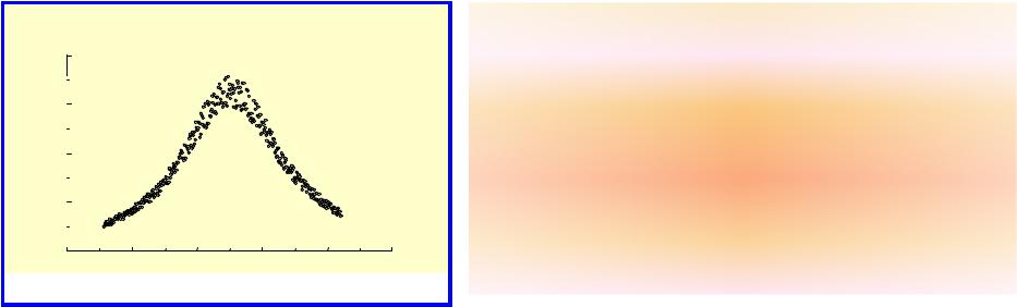
This figure represents a typical example. The presented data are measured in the limited interval of a variable x, contain the error of

measurements and could be fitted reasonably well either by a gaussian or some lorentzian contour. However, the careful investigation shows that this curve is neither a Gaussian nor Lorentzian. The best fitting can be realized with

	the help of the function R(x; A) = B xμ exp(-a x-
			1
	a x2/2) with B=1.55, μ = 0.6, a =1.5, a = 0.3.
	2	1	2

In spite of the fact that the linear least square method (LLSM) and its

possible generalizations is considered in many books nevertheless some interesting problems (even in one-dimensional regression task) are

remained unsolved. In this lecture we consider the eigen-coordinates (ECS) method that helps to reduce the problem of the fitting of a wide class of non-linear functions (when the fitting vector θ enters to by non-linear way) to the well-known LLSM.

6

POLS-Procedure of the Optimal Linear Smoothing

N

x − x

∑K

i

j

ninj

w

j=1

2

y = Gsm(x, nin, w) =

,

K(t) = exp(−t

)

N

x

− x

j

∑K

i

w

j=1

nj = Gsm(x, yj , w') −Gsm(x, yj , w), w' < w,

n(w))

100%.

min(RelErr(w)) = stdev(

mean( y(w))

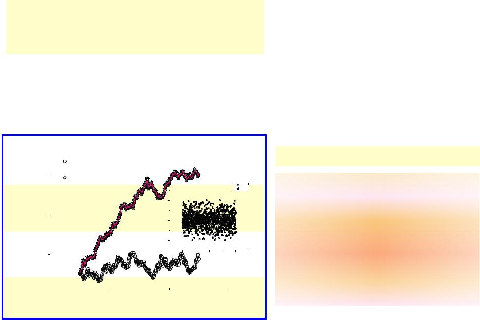
Here we want to mark also the following fact that was noticed from analysis of model data. If the initial random sequence determined as rndj does not have a trend then the first local minima is absent. So, in these cases it is preferable to create a trend artificially by numerical integration of the initial trend by the trapezoid method. After integration which is realized by means of the recurrence relationship

Jninj = Jninj−1 +0.5 (xj − xj−1 ) (rnd j−1 + rnd j )

We show the effect of creation a trend by means of integration procedure. The initial random sequences shown on the right-hand side do not have a trend. A possible trend coincides with OX axis. After integration by means of expression (5) we obtained the curves with clearly expressed trends that are shown on the central figure. The solid lines show the smoothed curves obtained by means of the POLS. The value of the optimal window equals approximately wopt 0.5.

7

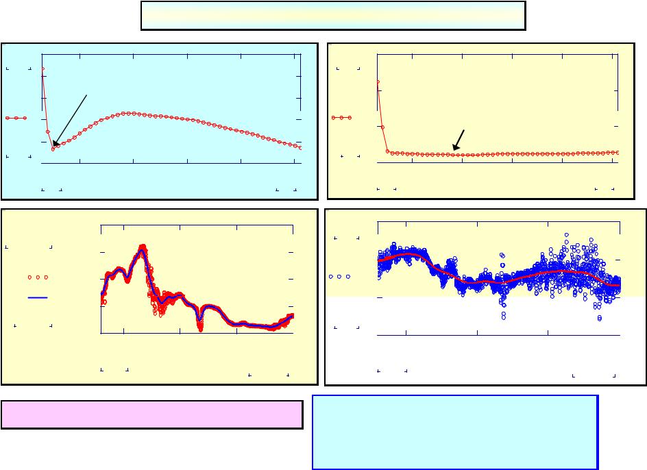
Procedure of the optimal linear smoothing (POLS)

W=0.05
.	.	.	.	.

	W=0.17
.	.	0.3	0.4	0.5
	wi			0.51

.

POLS allows to find an optimal trend!

		3	3×103
		wv	3
			3.996×10

Raoul R. Nigmatullin, Dumitru Baleanu, Erdal Dinch, and

Ali Osman Solak, "Characterization of a benzoic acid modified glassy carbon electrodes expressed

quantitatively by new statistical parameters." Physica E
41 (2009) 609-614.	8

8

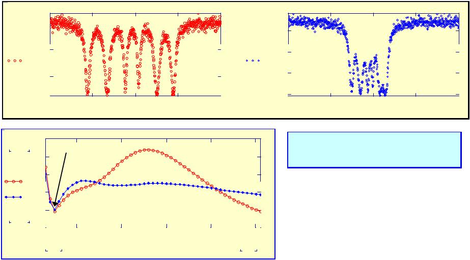
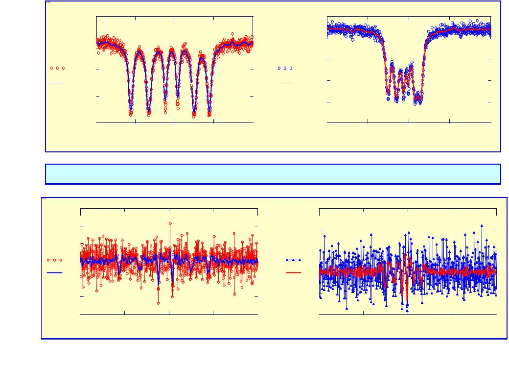
Initial Mossbauer spectra

4	6
v

W=0.051

POLS in action. Optimization of the smoothing procedure

9

.
4	6
v

	Demonstration of the POLS for the initial M-spectra and the spectra of the 2-nd order.
	4	6
	v	10
		10