

Anti-solvent unit
.pdfICheaP-8
The 8th International Conference on
Chemical & Process Engineering
ISCHIA Island Gulf of Naples 2427 June 2007
Optimal control of particle size in antisolvent crystallization operations
Seyed Mostafa Nowee1, Ali Abbas2, Jose A. Romagnoli3
1School of Chemical and Biomolecular Engineering, University of Sydney, Australia. 2School of Chemical and Biomedical Engineering, Nanyang Technological University, Singapore.
3Department of Chemical Engineering, Louisiana State University, USA.
In this paper we present a detailed antisolvent crystallization model. A population balance approach is adopted to describe the dynamic change of particle size in crystallization processes under the effect of antisolvent addition. The sodium chloride-water-ethanol is used as a model system. Maximum likelihood method is used to identify the nucleation and growth kinetic models for sodium chloride from data derived from controlled experiments. A number of growth and nucleation kinetic models are investigated in the estimation step to identify one with better prediction. The model is then validated under a new ethanol (antisolvent) addition profile showing to be in good agreement. The resulting model is then exploited in model-based optimization to readily develop optimal antisolvent feeding recipes. Two objective functions are used related to the control of particle size. Different feeding profiles are readily determined for different end-product particle size targets. The dynamic optimization results are successfully validated experimentally showing very close agreement. The approach presented here is rapid and repeatable and thus attractive for pharmaceutical and fine chemicals antisolvent crystallization operations aimed at control of particle size.
1. Introduction
Antisolvent crystallization (AC) operations are employed ubiquitously in the pharmaceutical and fine chemicals industries, producing solid particulate products. The particle size of the crystallization product is an important property that is typically required to conform to quality as well as operational demands. Particle size control is the concern of this paper in which we propose and present a model-based approach to optimal AC operation. In AC a secondary solvent known as antisolvent or precipitant is added to the solution resulting in the reduction of the solubility of the solute in the original solvent and consequently supersaturation is generated. The rate of supersaturation generation in AC is highly dependent on antisolvent addition rate. Keeping the supersaturation constant during a crystallization operation has been a long-standing technique for arguably optimal operation (Mullin and Nyvelt, 1971; Jones and Mullin, 1974). Zhou et al. (2006) have carried out concentration controlled seeded AC of a pharmaceutical compound using an algebraic equation for the solubility as a function of solvent. The main objective of their feedback
concentration control system was to keep the supersaturation low and constant. (Nonoyama et al., 2006) presented a simulation study on seeded solvent crystallization of an active pharmaceutical ingredient (API) by water addition to original solution. (Muhrer et al., 2002) provided a simplified model of the Gas Antisolvent (GAS) crystallization process that describes the vapor-liquid equilibrium as well as particle formation and growth. They validated the developed model and suggested its use as a tool to design and optimize GAS crystallization processes. In spite of all the previous works, there still exists a big gap in the systematic control of the product crystal size and other properties in antisolvent mediated crystallization. Model-based optimization to determine optimal AC strategies/recipes is poised to fill this gap and as far as the authors are aware, is not currently addressed.
In this paper, we outline how the developed model, which is based on the population balance theory, is 1) used in optimization-based parameter estimation to arrive at the nucleation and growth kinetic sub-model, and 2) utilized in model-based optimization to readily develop optimal antisolvent feeding recipes. A couple of objective functions related to the control of particle size are used, and different feeding profiles are readily determined for different end-product particle size targets. The dynamic optimization results are successfully validated experimentally showing very close agreement. The approach presented here is rapid and repeatable and thus attractive for pharmaceutical and fine chemicals AC operations aimed at control of particle size.
2. Modeling and kinetic parameter estimation
2.1 Theory
We present extensions to previously developed population balance based models (Abbas, 2003; Nowee et al., 2006), and address antisolvent effects and interactions. A summary of the model is given here while details will be presented in a full paper elsewhere. For a crystallization system with crystal growth assumed to be non-dispersed and independent of crystal size and where agglomeration and attrition are considered negligible, the population balance equation simplifies to:
∂n(L,t) |
= −G |
∂n(L,t) |
+ B − |
n(L,t) dV |
(1) |
∂t |
∂L |
V dt |
|
where n(L,t) is the number density of crystals, t is time, L is the characteristic crystal size, V is the suspension volume, G is the growth rate of the crystals and B is the nucleation rate which is equal to zero for all sizes but the first. The kinetic equations are:
B = kb |
C b M T |
(2) |
|
G = k |
|
C g |
(3) |
|
|
|
|
|
g |
C* |
|
where C is the absolute supersaturation, C* is the saturated concentration, MT is the magma density, kb and b are the nucleation parameters. In this growth rate power law model
structure, the parameters kg and g are defined as functions of antisolvent mass fraction in solute free mixture (z):
kg =k0 +k1z +k2 z2 |
(4) |
g = g0 + g1z |
(5) |
To complete the model, a solubility model (Yeo et al., 2007) and total and component mass balances are incorporated. As such, changes in suspension volume are evaluated by:
dV |
= |
dVL |
+ |
dVS |
(6) |
|
dt |
dt |
dt |
||||
|
|
|
Accordingly the numerator of equation (6) bears the antisolvent mass addition term as well as total solute mass in liquid phase. The antisolvent mass addition rate will become the optimization (time-varying) decision variable as will be discussed in Section 3. The model was implemented and solved in gPROMS (Process Systems Enterprise Ltd, UK).
The kinetic sub-model (Equations 2-5) contains a vector θ of parameters [kb, k0, k1, k2, b, g0, g1] that needs to be determined via a parameter estimation step. In recent years, rigorous parameter estimation methods have been employed in crystallization kinetics identification but of all techniques, posing the estimation as an optimization problem has been regarded as most relevant (Rawlings et al., 1993; Mignon et al., 1996). Essentially the parameter estimation problem is an optimization one where the model is fitted to the experimental data. Once parameters are estimated, the identified model may be used for predictive simulation analysis where the various operational variables may be studied, and for optimization and control scheme development. In this work, a maximum likelihood optimization is carried out using the gEST facility in gPROMS. The kinetic parameter set that provides the highest probability of the model predicting the real data is determined. For the estimation exercise, the measured crystallization system states are mean particle size and particle free solution density. In previous works, we successfully applied this method to the identification of ammonium sulfate kinetics for crystallizations under cooling mode of operation (Abbas, 2003; Nowee et al., 2006). The same method is applied here with differences being modifications in the current model and experimental conditions to describe AC under constant temperature.
2.2 Experimental
For the estimation step and kinetic model identification, four experiments were conducted under three different constant antisolvent feeding rates – one experiment at a feedrate of 194 ml.hr-1, two at a medium rate of 98.4 ml.hr-1 and one at a lower rate of 50 ml.hr-1. Figure 1 shows the schematic of the experimental apparatus, instrumentation and control system used. Analytical grade chemicals were used. Ethanol was added to the aqueous NaCl solution using a calibrated digital dosing pump (Grundfos, Denmark). The ethanol addition profile was implemented and controlled from within a distributed control system (DCS) environment (Honeywell, USA). Temperature was controlled, at 25°C for all experiments,
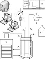
using a Pt100 thermo couple connected to heating/cooling circulator (Lau da, Germany ). Particle ch ord length was measured online every 2 seconds using focused be am reflectan ce measurement (FBRM) probe (Mettler-Toledo Lasentec Products, USA). Infrequent samples were rem oved iso-kinetically from the crystallizer for particle size and density measurements. Particle size was measured offline using Mastersizer 2000 particle si ze analyzer (Malvern Instruments, UK) while density was measure using an offline density
meter (An ton Paar D MA 5000, Au stria) after the samples |
was filtered |
u sing a syrin ge |
|
microfilte r. The concen tration of the solution was inferred from the density |
reading usi ng |
||
the correla tion of (Galle guillos et al., 2003). |
|
|
|
Fig . 1: Exp erimental |
Setup. A - |
||
Cr ystallization |
vessel, B |
- |
Temperature |
co ntrol system, C - Pt100 thermocouple, D - |
|||
Et hanol addition |
line, E - Pu mp, F - Ethanol |
||
reservoir, G - F BRM probe, H - Analog ue ou tput card, I - FBRM contro l computer, J - DC S Station, K - Controller I/O terminals, L - D CS server, M - Feed profile to pump.
2.3 Estimation results and model validation
In the mo del identification, we took a further step and compute d θ for four e mpirical growth kinetic su b-model structures:
• |
Model 1: Growth k inetic model is a function of absolute s upersaturation ( C) and t he |
|
|
param eters of Grow th (kg and g) are constant. |
C/C*) and t he |
• |
Model 2: Growth kinetic model is a function o f relative supersaturation ( |
|
|
param eters of Grow th (kg and g) are constant. |
|
• |
Model 3: Growth k inetic model is a function of absolute s upersaturation ( C) and t he |
|
|
param eters of Gro wth are functions (Equation s 4 and 5) of antisolvent |
mass fraction in |
|
solute free mixture. |
C/C*) and t he |
• |
Model 4: Growth kinetic is a function of relative supe rsaturation ( |
|
|
param eters of Gro wth are functions (Equation s 4 and 5) of antisolvent |
mass fraction in |
|
solute free mixture. |
|
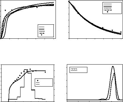
The estimation activities for all four sub-models were executed successfully. The goodness of the fits varied across the four mo dels with Mo del 4 being a dopted for further simulati on and optimization. Typic al estimation results in the form of overl ay plots are shown in Fig. 2. In a further exercise, we undertook the testing of the AC d ynamic predi ctions with t he adopted kinetic model. A totally ne w and non-co nstant feedrate of antisolve nt was defin ed arbitrarily and impleme nted. Figure 3 shows this feedrate profile along with the mean si ze profiles of experiment v ersus model prediction. A good agreem ent was found.
|
140 |
|
|
|
|
|
|
|
300 |
|
|
|
|
|
|
|
|
|
|
|
|
|
|
|
|
|
|
|
|
|
|
|
120 |
|
|
|
|
|
|
|
|
|
|
|
|
|
Model 1 |
|
|
|
|
|
|
|
|
|
|
|
|
|
|
Model 2 |
|
|
|
|
|
|
|
|
|
|
250 |
|
|
|
|
|
Model 3 |
|
100 |
|
|
|
|
|
|
|
|
|
|
|
|
|
Model 4 |
(micron) |
|
|
|
|
|
|
|
|
|
|
|
|
|
Experiment |
|
|
|
|
|
|
|
|
(gr/Ltr) |
|
|
|
|
|
|
||
|
|
|
|
|
|
|
200 |
|
|
|
|
|
|
||
Size |
80 |
|
|
|
|
|
|
solute |
|
|
|
|
|
|
|
60 |
|
|
|
|
|
|
150 |
|
|
|
|
|
|
||
|
|
|
|
|
|
|
|
|
|
|
|
|
|
|
|
Mean |
40 |
|
|
|
|
Model 1 |
|
C |
100 |
|
|
|
|
|
|
|
|
|
|
|
|
|
|
|
|
|
|
|
|||
|
|
|
|
|
Model 2 |
|
|
|
|
|
|
|
|
|
|
|
|
|
|
|
|
|
|
|
|
|
|
|
|
|
|
|
20 |
|
|
|
|
Model 3 |
|
|
50 |
|
|
|
|
|
|
|
|
|
|
|
Model 4 |
|
|
|
|
|
|
|
|
||
|
|
|
|
|
|
|
|
|
|
|
|
|
|
||
|
|
|
|
|
|
Experiment |
|
|
|
|
|
|
|
|
|
|
0 |
|
|
|
|
|
|
|
0 |
|
|
|
|
|
|
|
0 |
20 |
40 |
60 |
80 |
100 |
120 |
|
0 |
20 |
40 |
60 |
80 |
100 |
120 |
Time (min) |
Time (min) |
Figure 2: Results of Experiment 2 at antisolvent addition of 98.4 ml.hr-1. Overlay plots of experimental mean size (left) and solution concentration (right) against model predictions using the different kinetic models.
|
180 |
|
|
|
|
|
6 |
|
|
|
|
160 |
|
|
|
|
|
|
|
|
10 |
|
|
|
|
|
|
|
|
|
|
|
|
|
|
|
|
|
|
5 |
|
|
|
|
140 |
|
|
|
|
|
|
|
|
8 |
|
|
|
|
|
|
|
|
|
|
|
Mean Size (micron) |
120 |
|
|
|
|
|
4 |
Feed Rate (ml/min) |
Volume Percentage |
|
100 |
|
|
|
|
Mean Size (Expt) |
|
6 |
|||
|
|
|
|
Mean Size (Model) |
|
|
||||
|
|
|
|
|
3 |
|
||||
|
|
|
|
|
Ethanol Feed Rate |
|
||||
80 |
|
|
|
|
|
|
||||
|
|
|
|
|
|
4 |
||||
|
|
|
|
|
|
|
||||
60 |
|
|
|
|
|
2 |
|
|||
|
40 |
|
|
|
|
|
|
|
|
2 |
|
|
|
|
|
|
|
1 |
|
|
|
|
20 |
|
|
|
|
|
|
|
|
|
|
0 |
|
|
|
|
|
0 |
|
|
0 |
|
|
|
|
|
|
|
|
0.01 |
||
|
0 |
50 |
100 |
150 |
200 |
250 |
300 |
|
|
Model 4
Experiment
0.1 |
1 |
10 |
100 |
1000 |
Time (min) |
Size (μ) |
Figure 3: Experimental validation results showing the model prediction versus experimental data for mean size profile (left) and CSD (right) under a new antisolvent feedrate profile.
3. Model-based optimization
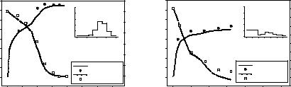
The mathematical description of the proposed dynamic optimization problem (DOP) can be summarized in Equation 7 inclusive of constraints of various types (Nowee et al., 2006). The objective function is simply the magnitude of a variable z(t), evaluated at the end of the optimization horizon t=tf. The results reported here correspond to two objective functions:
(1) maximization of final mean size, and (2) achievement of desired final mean size of 100 μm. The dynamic optimal mean size profiles and the corresponding concentration trends for both cases are presented in Figure 4. We further validate these profiles experimentally and found very good agreements with the optimization.
The model-based approach presented here allows systematic and rapid process development of optimal operation of AC generic to be readily implemented for control of particle size of pharmaceuticals or fine chemicals compounds.
Optimize z(t f ) |
|
|
|
|
|
|
|
|
|
|
|
||||||
t,u(t ),v,t [0,t f ] |
|
|
|
|
|
|
|
|
|
|
|
|
|
||||
|
|
|
|
& |
|
|
|
|
|
|
|
|
|
|
|
|
|
F(x(t), x(t), y(t),v) = 0;t [0,t f ] |
|
|
|
|
|
||||||||||||
& |
|
|
|
|
|
|
|
|
|
|
|
|
|
|
|
|
|
l(x(0), x(0), y(0),v) = 0 |
|
|
|
|
|
|
|
|
|
||||||||
t minf |
≤ t f |
≤ t maxf |
|
|
|
|
|
|
|
|
|
|
|
||||
u min (t) ≤ u(t) ≤ u max (t),t [0,t f ] |
|
|
|
|
|
||||||||||||
vmin (t) ≤ v ≤ vmax |
|
|
|
|
|
|
|
|
|
|
|
||||||
wmin |
|
≤ w(t |
f |
) ≤ w |
|
|
|
|
|
|
|
|
|
|
|
||
el |
|
|
|
|
el |
|
|
|
|
|
|
|
|
|
|
|
|
w (t |
f |
) = wtgt |
|
|
|
|
|
|
|
|
|
|
|
||||
ee |
|
|
|
|
ee |
|
|
|
|
|
|
|
|
|
|
|
|
wmin |
(t) ≤ w(t) ≤ w |
(t),t [0,t |
f |
] |
|
|
|
|
|
||||||||
tt |
|
|
|
|
|
tt |
|
|
|
|
|
|
|
|
|
||
wmin (t) ≤ w(t) ≤ wmax (t),t [0,t f ] |
|
|
|
|
|
||||||||||||
160 |
|
|
|
|
|
|
|
|
|
|
|
|
|
|
350 |
|
160 |
140 |
|
|
|
|
|
|
|
Feed Rate (ml/min) |
10 |
|
|
|
|
|
300 |
|
140 |
|
|
|
|
|
|
|
8 |
|
|
|
|
|
|
||||
|
|
|
|
|
|
|
|
|
|
|
|
|
|
|
|
||
120 |
|
|
|
|
|
|
|
6 |
|
|
|
|
|
250 |
Concentration (gr/Ltr) |
120 |
|
|
|
|
|
|
|
|
|
4 |
|
|
|
|
|
|
|||
|
|
|
|
|
|
|
|
|
|
|
|
|
|
100 |
|||
100 |
|
|
|
|
|
|
|
2 |
|
|
|
|
|
200 |
|||
|
|
|
|
|
|
|
|
|
|
|
|
|
|
||||
|
|
|
|
|
|
|
|
0 |
|
|
|
|
|
|
|||
80 |
|
|
|
|
|
|
|
|
|
|
|
|
|
80 |
|||
|
|
|
|
|
|
|
0 |
50 |
|
100 |
150 |
200 |
|
||||
|
|
|
|
|
|
|
|
|
150 |
|
|||||||
|
|
|
|
|
|
|
|
|
|
Time (min) |
|
|
|||||
60 |
|
|
|
|
|
|
|
|
|
|
|
60 |
|||||
|
|
|
|
|
|
|
|
|
|
|
|
|
|
||||
SizeMeanμ)( |
|
|
|
|
|
|
|
|
|
|
|
|
|
100 |
SizeMeanμ() |
||
40 |
|
|
|
|
|
|
|
|
|
|
|
|
|
|
|
Solute |
40 |
20 |
|
|
|
|
|
|
|
|
|
|
|
Mean Size (model) |
50 |
20 |
|||
|
|
|
|
|
|
|
|
|
|
|
Mean Size (expt) |
|
|
||||
|
|
|
|
|
|
|
|
|
|
|
|
|
|
|
|||
0 |
|
|
|
|
|
|
|
|
|
|
|
Solute Conc. (model) |
0 |
|
0 |
||
|
|
|
|
|
|
|
|
|
|
|
Solute Conc. (expt) |
|
|||||
|
|
|
|
|
|
|
|
|
|
|
|
|
|
|
|||
|
|
|
0 |
|
50 |
100 |
150 |
200 |
250 |
|
300 |
|
350 |
|
|
|
|
(7)
|
|
|
|
|
|
|
|
|
|
|
|
320 |
|
|
|
|
|
Feed Rate (ml/min) |
10 |
|
|
|
|
|
|
300 |
|
|
|
|
|
8 |
|
|
|
|
|
|
|
||
|
|
|
|
|
|
|
|
|
|
|
|
||
|
|
|
|
6 |
|
|
|
|
|
|
280 |
Concentration (gr/Ltr) |
|
|
|
|
|
|
|
|
|
|
|
|
|||
|
|
|
|
4 |
|
|
|
|
|
|
260 |
||
|
|
|
|
|
|
|
|
|
|
|
|||
|
|
|
|
2 |
|
|
|
|
|
|
240 |
||
|
|
|
|
0 |
|
|
|
|
|
|
|||
|
|
|
|
|
|
|
|
|
|
|
|||
|
|
|
|
0 |
10 |
20 |
30 |
40 |
50 |
60 |
220 |
||
|
|
|
|
|
|
Time (min) |
|
|
|||||
|
|
|
|
|
|
|
|
|
|||||
|
|
|
|
|
|
|
|
|
|
|
200 |
||
|
|
|
|
|
|
|
|
|
|
|
|
||
|
|
|
|
|
|
|
|
|
|
|
|
180 |
Solute |
|
|
|
|
|
|
|
Mean Size (model) |
160 |
|||||
|
|
|
|
|
|
|
Mean Size (expt) |
|
|||||
|
|
|
|
|
|
|
Solute Conc. (model) |
140 |
|
||||
|
|
|
|
|
|
|
Solute Conc. (expt) |
|
|||||
|
|
|
|
|
|
|
|
|
|
|
|
120 |
|
0 |
20 |
40 |
60 |
|
80 |
|
|
100 |
|
|
120 |
|
|
Time (min) |
Time (min) |
Figure 4: Optimal feedrate and experimental validation of mean size and concentration results under objective function (1) (left) and objective function (2) (right).
5. References
Abbas, A., 2003, PhD Dissertation, University of Sydney, 2003.
Galleguillos, H.R., M.E. Taboada, T.A. Graber and S. Bolado, 2003, J. Chem. Eng. Data, 48, 405-410.
Jones, A.G. and J.W. Mullin, 1974, Chem. Eng. Sci., 29, 105-118.
Mignon, D., T. Manth and H. Offermann, 1996, Chem. Eng. Sci., 51, 2565-2570. Muhrer, G., C. Lin and M. Mazzotti, 2002, Ind. Eng. Chem. Res., 41, 3566-3579. Mullin, J.W. and J. Nyvelt, 1971, Chem. Eng. Sci., 26, 369-377.
Nonoyama, N., K. Hanaki and Y. Yabuki, 2006, Org. Process Res. Dev., 10, 727-732. Nowee, S.M., A. Abbas and J.A. Romagnoli, 2007, Chem. Eng. Process. 46, 1096-1106, Rawlings, J.B., S.M. Miller and W.R. Witkowski, 1993, Ind. Eng. Chem. Res., 32, 1275-96. Yeo, P., A. Abbas, S.M. Nowee and J.A. Romagnoli, 2007, In Preparation.
Zhou, G.X., M. Fujiwara, X.Y. Woo, E. Rusli, H.H. Tung, C. Starbuck, O. Davidson, Z. Ge and R.D. Braatz, 2006, Cryst. Growth Des., 6, 892-898.