pvt

PVT Analysis for Compositional Simulation

Steve Furnival

Roxar Oxford

February 2000

PVT Analysis

Roxar Oxford

2

12/12/12

PVT Analysis

Table of Contents

Table of Contents................................................................................................................					3
Table of Figures ..................................................................................................................					6
1.	Introduction ..................................................................................................................				7
2.	Hydrocarbon Composition ...........................................................................................				9
	2.1	The Atom...............................................................................................................			9
	2.1.1		The Carbon Atom .........................................................................................		10
	2.2	Basic Hydrocarbon Molecules – the Alkanes......................................................			10
	2.2.1		Isomerism......................................................................................................		13
	2.2.2		Alkenes and Alkynes ....................................................................................		14
	2.3	Cycloalkanes........................................................................................................			15
	2.4	Aromatics.............................................................................................................			16
	2.5	Polyaromatics ......................................................................................................			17
	2.6	Other Compounds................................................................................................			17
	2.7	Single Carbon Number Groups ...........................................................................			17
	2.7.1 Generalized SCN Physical Properties...........................................................				18
	2.8	The Plus Fraction.................................................................................................			19
3.	Phase Behaviour.........................................................................................................				21
	3.1	Pure Component Phase Behaviour ......................................................................			21
	3.1.1		p-T Projection................................................................................................		23
	3.1.2		p-V Projection ...............................................................................................		24
	3.2	Binary Mixture Phase Behaviour ........................................................................			25
	3.3	Multi-Component Base Behaviour......................................................................			27
	3.3.1 Dry and Wet Gas...........................................................................................				28
	3.3.2		Gas Condensates ...........................................................................................		28
	3.3.3		Volatile Oils..................................................................................................		30
	3.3.4		Crude Oils .....................................................................................................		30
	3.4	The Corresponding States Theorem ....................................................................			31
	3.4.1		Z-Factor Correlations....................................................................................		33
		3.4.1.1		Estimating Pseudo-Criticals ......................................................................	34
4. Sampling and Laboratory Analysis............................................................................					35
	4.1	Sampling..............................................................................................................			35
	4.1.1		Well Testing..................................................................................................		35
	4.1.2		Conditioning .................................................................................................		36
	4.1.3		Down Hole Sampling....................................................................................		36
	4.1.4		Surface Sampling..........................................................................................		38
		4.1.4.1 Liquid Loading in Gas Wells.....................................................................			38
		4.1.4.2		Taking Samples .........................................................................................	39
		4.1.4.3		Metering.....................................................................................................	39
		4.1.4.4		Checking the Data .....................................................................................	41
		4.1.4.5		Recombination Example............................................................................	41
	4.2	Laboratory Analysis ............................................................................................			45
	4.2.1		Compositional Determination.......................................................................		45

Roxar Oxford

3

12/12/12

PVT Analysis

	4.2.2		Saturation Pressure (SAT) ............................................................................	47
		4.2.2.1 The PVT Cell.............................................................................................		47
	4.2.3 Constant Composition Expansion (CCE) .....................................................			50
	4.2.4		Separator Test (SEP).....................................................................................	51
	4.2.5		Differential Liberation (DLE).......................................................................	52
	4.2.6 Constant Volume Depletion (CVD)..............................................................			54
		4.2.6.1 CVD Material Balance Check ...................................................................		55
	4.2.7		Other Experiments ........................................................................................	56
5.	Equations of State ......................................................................................................			59
	5.1	Development of the Ideal Gas Law .....................................................................		59
	5.1.1		The Mole.......................................................................................................	60
	5.1.2 Deficiencies in the Ideal Gas Law ................................................................			61
	5.1.3 The Real Gas Law.........................................................................................			61
	5.2	Cubic EoS............................................................................................................		62
	5.2.1 Van der Waals EoS .......................................................................................			62
	5.2.2 Redlich-Kwong Family of EoS.....................................................................			64
		5.2.2.1 Zudkevitch Joffe RK EoS..........................................................................		64
		5.2.2.2 Soave RK EoS ...........................................................................................		65
	5.2.3		Peng-Robinson EoS ......................................................................................	65
	5.2.4 The Martin’s 2-Parameter EoS .....................................................................			66
	5.2.5		Other Cubic EoS ...........................................................................................	66
	5.3	Multi-Component Systems..................................................................................		67
	5.4	Volume Translation .............................................................................................		68
6.	Flash Calculations ......................................................................................................			69
	6.1	Successive Substitution (SS) Method..................................................................		70
	6.1.1		Rachford-Rice Equation................................................................................	72
	6.2	Stability Test........................................................................................................		73
	6.3	Saturation Pressure ..............................................................................................		74
	6.4	Composition versus Depth...................................................................................		75
7.	Characterization .........................................................................................................			77
	7.1	Molar Distribution Models ..................................................................................		77
	7.1.1		Quadrature.....................................................................................................	79
	7.1.2		Modified Whitson Method............................................................................	80
	7.2	Inspection Properties Estimation .........................................................................		81
	7.3	Critical Property Estimation ................................................................................		83
	7.3.1 Normal Boiling Point Temperature ..............................................................			83
	7.3.2 Critical Temperature, Critical Pressure.........................................................			83
	7.3.3		Critical Volume.............................................................................................	84
	7.3.4		Acentric Factor..............................................................................................	84
8.	Regression ..................................................................................................................			85
	8.1	Objective Function ..............................................................................................		85
	8.2	Variable Choice ...................................................................................................		87
	8.3	Constraints...........................................................................................................		88
9.	Export for Simulation.................................................................................................			89
	9.1	Black Oil Modeling .............................................................................................		89
	9.2	Compositional Modeling .....................................................................................		92

Roxar Oxford

4

12/12/12

PVT Analysis

9.2.1		Grouping .......................................................................................................	92
9.2.2		Mixing Rules .................................................................................................	93
References		.........................................................................................................................	95
Appendix A: Classical Thermodynamics .........................................................................			97
A.1	Abstractions.........................................................................................................		97
A.2	Chemical ...............................................................................................Potential		98
A.2.1 .........................................................................................................		Fugacity	99
A.3	Equilibrium........................................................................................................		100

Roxar Oxford

5

12/12/12

PVT Analysis

Table of Figures
Figure 1: The Total Production System..............................................................................	7
Figure 2: Schematic of Methane Molecule showing four C-H Bonds..............................	10
Figure 3: Schematic of Ethane Molecule..........................................................................	11
Figure 4: Schematic of Propane Molecule........................................................................	11
Figure 5: Schematic Representations of Butane Isomers, nC4 and iC4.............................	13
Figure 6: Schematic Representation of Pentane Isomers..................................................	13
Figure 7: Schematic of the Alkene Double Bond. ............................................................	14
Figure 8: Schematic of the Alkyne Triple Bond...............................................................	15
Figure 9: Schematic Representation of Cyclopentane and Cyclohexane. ........................	16
Figure 10: Alternate Schematic Representations for Benzene Molecule .........................	16
Figure 11: The p-V-T Behaviour of a Pure Substance. [From Adkins] ............................	22
Figure 12: p-T and p-V projections from the 3D p-V-T Surface [from Adkins]...............	23
Figure 13: p-T Projection for a Pure Component..............................................................	23
Figure 14: p-V Projection for a Pure Component .............................................................	25
Figure 15: Phase Envelopes of C2-C10 Binary Mixtures...................................................	26
Figure 16: Multi-Component Phase Envelope..................................................................	27
Figure 17: Schematic Phase Envelope of a Dry and Wet Gas..........................................	28
Figure 18: Liquid Dropout Profile from Gas Condensate [at constant composition].......	29
Figure 19: Standing Z-Factor Chart..................................................................................	32
Figure 20: Schematic of the Venturi Tube Rate Measurement.........................................	39
Figure 21: Schematic of an Orifice Plate Gas Rate Device ..............................................	39
Figure 22: Surface Separator Analysis. ............................................................................	42
Figure 23: Standing Analysis for the Separator Stage......................................................	44
Figure 24: Schematic of a GC System..............................................................................	45
Figure 25: Schematic of the FID [from www.scimedia.com]. .........................................	46
Figure 26: Freezing point depression diagram [from Pedersen et al.]..............................	47
Figure 27: Schematic of a Gas Condensate PVT cell.......................................................	48
Figure 28: Change in Slope of p-V curve around the Bubble Point. ................................	48
Figure 29: Liquid Dropout “Tail” Shown by Some Gas Condensates .............................	49
Figure 30: Schematic of CCE applied to Gas Condensate Fluid......................................	50
Figure 31: Schematic of 2-Stage Separator Test...............................................................	51
Figure 32: Schematic of Differential Liberation Experiment...........................................	53
Figure 33: Schematic of CVD Performed on Gas Condensate Fluid ...............................	54
Figure 34: Schematic of the Swelling Test.......................................................................	57
Figure 35: Schematic of the Slim Tube Apparatus [ref. See Figure 27]...........................	58
Figure 36: Charles’ Law Behaviour for Water Implying Zero Temperature....................	59
Figure 37: p-V Behaviour for Pure Component with Cubic EoS Behaviour....................	63
Figure 38: Flow Diagram for the Successive Substitution Flash......................................	71
Figure 39: Gas-Oil Contact...............................................................................................	76
Figure 40: Critical Transition............................................................................................	76
Figure 41: Whitson GDM for different values of ..........................................................	78
Figure 42: Schematic of the Generalized BO Table Construction. ..................................	90

Roxar Oxford

6

12/12/12

PVT Analysis

1.Introduction

In order to perform flow simulation in the reservoir and production system, we need to know various physical properties of the fluid system. Firstly, what phases are present? Gas? Oil? Water? What are the relative proportions of these phases? What are the bulk phase properties, i.e. density, viscosity, thermal conductivity, etc.

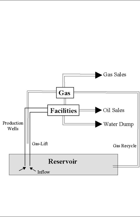
In principle, we can and do take samples of the reservoir fluid and measure the quantities of interest at certain pressures and temperature. However, these experiments are both difficult and costly and cannot hope to cover the range of pressures, temperatures and compositions we are likely to encounter. Consider the following schematic of the total production system:

Figure 1: The Total Production System.

In mature areas such as the North Sea, petroleum accumulations are being sought at evergreater depths: it is now common to find reservoirs at 20000-ft [6100 m] or more. At such depths, pressures can approach 16000 psia [1100 bars] and temperatures are close to 400 oF [205 oC]. Pressure can take any value between initial reservoir pressure and 1

Roxar Oxford

7

12/12/12

PVT Analysis

atmosphere in the stock tank, if one exists. Temperature will also vary between reservoir temperature and standard temperature although lower temperatures are possible in subsea flow lines and cryogenic coolers.

If the fluid composition was fixed, a set of pre-defined look-up tables could handle temperature and pressure variability. This is the black oil approach, which we will review later in this course.

Generally, the fluid composition within the production system is not fixed for a variety of reasons. Within the reservoir, the following changes can take place:

Composition varies with depth and areal location. The presence of high permeability streaks can then allow different fluids to mix.

As fluid drops below saturation pressure, one phase – generally the gas – will flow in preference to the oil so the produced well composition changes with time. This effect is particularly important for Gas Condensates and Volatile Oils – near critical fluids.

Gas injection for pressure maintenance or miscibility processes.

Within the production system:

Fluids from different parts of the reservoir or reservoirs, can mix, i.e. Eastern Trough Area Project (ETAP).

Gas injection for Gas-Lift.

Changes in surface separation.

Phase slippage in long pipe and flow lines can cause formation of liquid slugs.

All these cases, and more, point to the need for a compositional treatment of the fluid system. These methods are computational expensive. However, with the rapid increase in computer power at reducing cost, they are all now achievable on a high-end PC.

Roxar Oxford

8

12/12/12

PVT Analysis

2.Hydrocarbon Composition

Hydrocarbons are molecules1 composed principally of Hydrogen and Carbon but also containing Sulphur, Nitrogen, Oxygen and various trace metals.

Carbon is unique amongst the elements in its ability to form not only strong CarbonCarbon bonds but strong Carbon-OtherElement bonds also. Because of this ability, the number of naturally occurring molecules containing Carbon is vast. So much so that one of the main sub-disciplines within Chemistry is devoted to the study of Carbon compounds – Organic Chemistry. In order to appreciate the richness of Carbon compounds, it is worth taking a short time to understand the nature of how atoms bind within molecules.

2.1 The Atom

Consists of a central positively charged nucleus of +Z units, comprising the majority of the atom’s mass, surrounded by Z electrons, each of charge –1. Electrons are forced to occupy certain orbits or shells by the laws of quantum physics. The number of electrons that can occupy each shell is limited. The first can hold two, the second eight, etc. As the Z electrons are added to balance up the charge on the nucleus, they will fill the shells from the inside out.

When the outermost shell is not complete then the atomic species will try to bond with other atomic species to close the shell. Atomic species containing just one electron in their outermost shell, such as the Group I Alkali metals2 will donate their spare electron to atoms that are missing one in their outermost shell. Similarly, atoms such as the Group II Alkaline metals3 will donate their two spare electrons to atoms missing one or two electrons. Atoms missing one or two electrons in their outermost shell include the Group VII Halogens4 or Group VI atoms5. The exchange of electrons causes the donor become positively charged and the recipient ions to become negatively charged. The electrostatic attraction between the ions is what then provides the bonding mechanism. This is known as ionic bonding.

The other way in which atoms can close their outermost shell is by sharing electrons with other atomic species that have vacancies in the outermost shell. This is known as covalent bonding and is the mechanism that dominates Carbon chemistry.

1A molecule is the smallest sub-division of a chemical species which is representative of that species.

2Lithium, Sodium, Potassium, etc.

3Beryllium, Magnesium, Calcium, etc

4Fluorine, Chlorine, Bromine, etc.

5, Oxygen, Sulphur, etc.

Roxar Oxford

9

12/12/12

PVT Analysis

2.1.1 The Carbon Atom

The nucleus of the most commonly occurring Carbon consists, in part, of six positively charged protons. Therefore, its six electrons are arranged in two shells; the inner shell of two electrons is full and the outer shell of four electrons is four short of being complete. Therefore, each Carbon atom requires other atomic species to share four electrons with it. Note the four electrons required do not have to come from four other atoms. CarbonCarbon pairs can exchange one, 2 or 3 electrons with each other to form what are known as single, double and triple bonds. Naturally occurring hydrocarbons usually only consist of Carbon-Carbon pairs with single bonds.

These four other electrons can be donated by four other Carbon atoms in one of two different ways. When combined in a 2D planar lattice structure, the result is graphite - a soft powder that is used in pencils. When combined in a 3D tetrahedral structure, the result is diamond – an ultra-hard crystal that is prized for its durability.

When Carbon combines with other atomic species, principally hydrogen, the result is the series of chemical compounds found in petroleum.

2.2 Basic Hydrocarbon Molecules – the Alkanes

The most common hydrocarbon molecule by number is that of Methane. It consists of a single Carbon atom surrounded by 4 hydrogen atoms each of which shares its single electron thereby closing the Carbon outer shell of 8 and the single Hydrogen shell of 2. The Hydrogen atoms arrange themselves at the apexes of a tetrahedron with the Carbon atom at the centre of the structure. Symbolically Methane is represented by:

Figure 2: Schematic of Methane Molecule showing four C-H Bonds

The common shorthand representation is CH4: on PVT reports it will be denoted as C1.

If one of the C-H bonds is broken, the resulting Methyl radical is highly reactive and will look to fill the missing electron hole as quickly as possible. If another Methyl radical is close by, they will C-C bond to form Ethane, which is represented by:

Roxar Oxford

10

12/12/12