Radiation Physics for Medical Physiscists - E.B. Podgorsak

2.3 Bohr Model of the Hydrogen Atom

59

θmin and θmax of (2.36) and (2.41), respectively, into (2.54), we now get the

following expression for the mean square angle Θ2 in Rutherford scattering

= 2π ρ

NA

tD2

ln

1.4ao

Θ2

A

α

−

N

Ro

√AZ

3

NA

zZe2

2

1.4ao

= 2π ρ

ln

(2.55)

Ro

√AZ

,

A

4πεoEK

t

3

˚

where ao = 0.5292 A and Ro = 1.2 fm are the Bohr radius constant of (2.58) below and the nuclear radius constant of (1.14), respectively.

2.3 Bohr Model of the Hydrogen Atom

Niels Bohr in 1913 combined Rutherford’s concept of the nuclear atom with Planck’s idea of the quantized nature of the radiative process and developed an atomic model that successfully deals with one-electron structures such as the hydrogen atom, singly ionized helium, doubly ionized lithium, etc. The model, known as the Bohr model of the atom, is based on four postulates that combine classical mechanics with the concept of angular momentum quantization.

The four Bohr postulates are stated as follows.

1.Postulate 1: Electrons revolve about the Rutherford nucleus in welldefined, allowed orbits (often referred to as shells). The Coulomb force of

attraction Fcoul = Ze2/(4πεor2) between the electrons and the positively charged nucleus is balanced by the centripetal force Fcent = mυ2/r, where Z is the number of protons in the nucleus (atomic number); r the radius of the orbit or shell; me the electron mass; and υ the velocity of the electron in the orbit.

2.Postulate 2: While in orbit, the electron does not lose any energy despite being constantly accelerated (this postulate is in contravention of the basic law of nature which states that an accelerated charged particle will lose part of its energy in the form of radiation).

3.Postulate 3: The angular momentum L = meυr of the electron in an allowed orbit is quantized and given as L = n , where n is an integer referred to as the principal quantum number and = h/(2π) is the reduced Planck’s constant with h the Planck’s constant. The simple quantization of angular momentum stipulates that the angular momentum can have only integral multiples of a basic value ( ).

4.Postulate 4: An atom or ion emits radiation when an electron makes a transition from an initial allowed orbit with quantum number ni to a final allowed orbit with quantum number nf for ni > nf .

The angular momentum quantization rule simply means that is the lowest angular momentum available to the electron (n = 1, ground state) and that

60 2 Rutherford–Bohr Atomic Model

higher n orbits (n > 1, excited states) can only have integer values of for the magnitude of the orbital angular momentum, where n is the principal quantum number or the shell number. One-electron atomic structures are now referred to as the Bohr atom.

2.3.1 Radius of the Bohr Atom

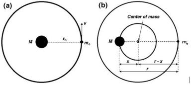
Assuming that Mnucleus ≈ ∞ and that Mnucleus melectron, equating the centrifugal force and the Coulomb force on the electron [see Fig. 2.5a]

meυ2	=		1		Ze2	(2.56)
rn		4πεo			rn2

and inserting the quantization relationship for the angular momentum of the electron (third Bohr postulate)

L = meυnrn = meωnrn2 = n ,

(2.57)

we get the following relationship for rn, the radius of the n-th allowed Bohr orbit

πε ( c)2

n2

n2

n2

rn =

4 o

= ao

= (0.5292 A)˚

×

, (2.58)

e2

mec2

Z

Z

Z

˚

where ao is called the Bohr radius of a one electron atom (ao = 0.5292 A).

2.3.2 Velocity of the Bohr Electron

Inserting the expression for rn of (2.58) into (2.57) we obtain the following expression for υn/c, where υn is the velocity of the electron in the n-th allowed

Fig. 2.5. Schematic diagram of the Rutherford–Bohr atomic model. In a the electron revolves about the center of the nucleus M where the nuclear mass M → ∞, in b the nuclear mass M is finite and both the electron as well as the nucleus revolve about their common center-of-mass

2.3 Bohr Model of the Hydrogen Atom

61

Bohr orbit

υ

n c

e2

1

Z

n

=

=

c

mec2rn

4πεo

c

n

n

,

(2.59)

= α

n

≈ 137

n

≈ (7 × 10−3) ×

Z

1

Z

Z

where α is the so-called fine structure constant ( 1/137).

Since, as evident from (2.59), the electron velocity in the ground state (n = 1) orbit of hydrogen is less than 1% of the speed of light c, the use of classical mechanics in one-electron Bohr atom is justifiable. Both Rutherford and Bohr used classical mechanics in their momentous discoveries of the atomic structure and the kinematics of electronic motion, respectively. On the one hand, nature provided Rutherford with an atomic probe (naturally occurring α particles) having just the appropriate energy (few MeV) to probe the atom without having to deal with relativistic e ects and nuclear penetration. On the other hand, nature provided Bohr with the hydrogen one-electron atom in which the electron can be treated with simple classical relationships.

2.3.3 Total Energy of the Bohr Electron

The total energy En of the electron when in one of the allowed orbits (shells) with radius rn is the sum of the electron’s kinetic energy EK and potential energy EP

mev2

Ze2

rn

dr

1 Ze2 1

Ze2 1

En = EK + EP =

n

+

=

−

=

2

4πεo

r2

2

4πεo

rn

4πεo

rn

∞

1 Ze2 1

1

e2

2

mec2

Z

2

Z

2

= −

= −

= −ER

=

2

4πεo

rn

2

4πεo

( c)2

n

n

Z

2

= (−13.61 eV) ×

.

(2.60)

n

Equation (2.60) represents the energy quantization of allowed bound electronic states in a one-electron atom. This energy quantization is a direct consequence of the simple angular momentum quantization L = n introduced by Bohr. ER is called the Rydberg energy (ER = 13.61 eV).

By convention the following conditions apply:

•A stationary free electron, infinitely far from the nucleus has zero energy.

•An electron bound to the nucleus can only attain discrete allowed negative energy levels, as predicted by (2.60).

•An electron with a positive energy is free and moving in a continuum of kinetic energies.

62 2 Rutherford–Bohr Atomic Model

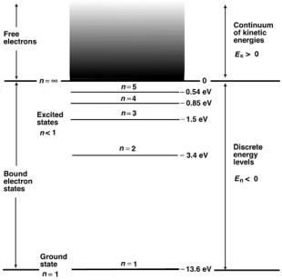
•The five lowest bound energy levels (n = 1 through n = 5) of the hydrogen atom according to (2.60) are: −13.6 eV, −3.4 eV, −1.51 eV, −0.85 eV, and −0.54 eV.

The energy level diagram for a hydrogen atom is shown in Fig. 2.6. It provides an excellent example of energy level diagrams for one-electron structures such as hydrogen, singly ionized helium atom, or doubly ionized lithium atom. The energy levels for hydrogen were calculated from (2.60) using Z = 1. The following features can be easily identified:

•The negative energy levels of the electron represent discrete allowed electron states bound to the nucleus with a given binding energy.

•The positive energy levels represent a free electron in a continuum of allowed kinetic energies.

•The zero energy level separates the discrete allowed bound electron states from the continuum of kinetic energies associated with a free electron.

•Electron in n = 1 state is said to be in the ground state; an electron in a state with n > 1 is said to be in an excited state.

•Energy must be supplied to an electron in the ground state of a hydrogen atom to move it to an excited state. An electron cannot remain in an

Fig. 2.6. Energy level diagram for the hydrogen atom as example of energy level diagrams for one-electron structures. In the ground state (n = 1) the electron is bound to the nucleus with a binding energy of 13.6 eV

2.3 Bohr Model of the Hydrogen Atom

63

excited state; rather it will move to a lower level shell and the transition energy will be emitted in the form of a photon.

2.3.4 Transition Frequency and Wave Number

The energy hν of a photon emitted as a result of an electronic transition from an initial allowed orbit with n = ni to a final allowed orbit with n = nf , where ni > nf , is given by

1

hν = Ei − Ef = −ERZ2

n2

−

n2

.

(2.61)

i

f

The wave number of the emitted photon is then given by

k = λ

= c

= 2π c Z2

nf2

− ni2

= R∞Z2

nf2

− ni2

=

1

ν

ER

1

1

1

1

= (109 737 cm−1) × Z2	1		1			(2.62)
			−		,
		n2		n2
		f		i

where R∞ is the so-called Rydberg constant (109 737 cm−1).

2.3.5 Atomic Spectra of Hydrogen

Photons emitted by excited atoms are concentrated at a number of discrete wavelengths (lines). The hydrogen spectrum is relatively simple and results from transitions of a single electron in the hydrogen atom. Table 2.1 gives a listing for the first five known series of the hydrogen emission spectrum. It

˚

also provides the limit in eV and A for each of the five series.

Table 2.1. Characteristics of the first five emission series of the hydrogen atom

Name of	Spectral	Final	Initial		Limit of	Limit of
series	range	orbit	orbit		series (eV)	˚
						series (A)
		nf	ni
Lyman	ultraviolet	1	2,3,4	. . . ∞	13.6	912
Balmer	visible	2	3,4,5	. . . ∞	3.4	3646
Paschen	infrared	3	4,5,6	. . . ∞	1.5	8265
Brackett	infrared	4	5,6,7	. . . ∞	0.85	14584
Pfund	infrared	5	6,7,8	. . . ∞	0.54	22957

64 2 Rutherford–Bohr Atomic Model

2.3.6 Correction for Finite Mass of the Nucleus

A careful experimental study of the hydrogen spectrum has shown that the Rydberg constant for hydrogen is 109 678 cm−1 rather than the R∞ = 109 737 cm−1 value that Bohr derived from first principles. This small discrepancy of the order of one part in 2000 arises from Bohr’s assumption that the nuclear mass (proton in the case of hydrogen atom) M is infinite and that the electron revolves about a point at the center of the nucleus, as shown schematically in Fig. 2.5a on page 60.

When the finite mass of the nucleus M is taken into consideration, both the electron and the nucleus revolve about their common center-of-mass, as shown schematically in Fig. 2.5b. The total angular momentum L of the system is given by the following expression:

L = me(r − x)2ω + M x2ω ,

(2.63)

where

ris the distance between the electron and the nucleus,

x is the distance between the center-of-mass and the nucleus, r − x is the distance between the center-of-mass and the electron.

After introducing the relationship

me(r − x) = M x

(2.64)

into (2.63), the angular momentum L for the atomic nucleus/electron system may be written as

	ω + me(r − x)2	meM
L = M x2		ω = me + M r2ω = µr2ω ,	(2.65)

where µ is the so-called reduced mass of the nucleus/electron system given as

µ =	meM	=	me		(2.66)
				.
	me + M		1 + me
			M

All Bohr relationships, given above for one-electron structures in (2.58) through (2.62) with a nuclear mass M → ∞, are also valid for finite nuclear masses M as long as the electron rest mass me in these relationships is replaced with the appropriate reduced mass µ.

For the hydrogen atom µ = me/(1 + me/Mproton) = 0.9995 me and the Rydberg constant RH is

µ

1

109 737 cm−1

= 109 677 cm−1 ,

RH =

R∞ =

R∞ =

me

1 +

me

1+

1

Mproton

1837

(2.67)

representing a 1 part in 2000 correction, in excellent agreement with the experimental result.

2.3 Bohr Model of the Hydrogen Atom

65

2.3.7 Positronium

The positronium “atom” (Ps) is a semi-stable, hydrogen-like configuration consisting of a positron and electron revolving about their common center-of- mass before the process of annihilation occurs. The lifetime of the positronium is about 10−7 s. The reduced mass µ for the positronium “atom” is me/2; the Rydberg constant RPs = R∞/2; the radius of orbits (rPs)n = 2aon2; and the ground state energy (EPs)n = ER/(2n2).

2.3.8 Muonic Atom

A muonic atom consists of a nucleus of charge Ze and a negative muon revolving about it. The muonic mass Mmuon is 207me. The reduced mass for a muonic atom with Z = 1 is 186me; the Rydberg constant Rmuon = 186R∞; and the ground state energy Emuon = 186ER.

2.3.9 Quantum Numbers

Bohr’s atomic theory predicts quantized energy levels for the one-electron hydrogen atom that depend only on n, the principal quantum number, since En = −ER/n2, where ER is the Rydberg energy.

In contrast, the solution of the Schr¨odinger’s equation in spherical coordinates for the hydrogen atom gives three quantum numbers for the hydrogen atom: n, , and m , where:

nis the principal quantum number with allowed values n = 1, 2, 3 . . ., giving the electron binding energy in shell n as En = −ER/n2,

is the orbital angular momentum quantum number with the following

	allowed values = 0, 1, 2, 3, . . . n − 1, giving the electron orbital angular
m	momentum L =		( + 1),
	is referred to as
	the orbital angular momentum Lz = m and has the following allowed
	values: m = − , − + 1, − + 2, . . . − 2, − 1, .
	Experiments by Otto Stern and Walter Gerlach in 1921 have shown that

the electron, in addition to its orbital angular momentum L, possesses an intrinsic angular momentum. This intrinsic angular momentum is referred

to as the spin S and is specified by two quantum numbers: s = 1/2 and

m that can take two values (1/2 or −1/2). The electron spin is given as

s √

S = s(s + 1) = 3/2 and its z component as Sz = ms .

•The orbital and spin angular momenta of an electron actually interact with one another. This interaction is referred to as the spin-orbit coupling

and results in a total electronic angular momentum J that is the vector

sum of the orbital and intrinsic spin components, i.e., J = L+S. The total

angular momentum J has the value J = j(j + 1) where the possible

66 2 Rutherford–Bohr Atomic Model

values of the quantum number j are:

| − s| , | − s + 1| , . . . | + s|, with s = 1/2 for all electrons.

•The z component of the total angular momentum has the value Jz = mj ,

where the possible values of mj are: −j, −j + 1, −j + 2, . . . j − 2, j − 1, j.

•The state of an atomic electron is thus specified with a set of four quantum numbers:

–n, , m , ms when there is no spin-orbit interaction

or

–n, , j, mj when there is spin-orbit interaction.

2.3.10 Successes and Limitations of the Bohr Atomic Model

With his four postulates and the innovative idea of angular momentum quantization Bohr provided an excellent extension of the Rutherford atomic model and succeeded in explaining quantitatively the photon spectrum of the hydrogen atom and other one-electron structures such as singly ionized helium, doubly ionized lithium, etc.

According to the Bohr atomic model, each of the five known series of the hydrogen spectrum arises from a family of electronic transitions that all end at the same final state nf . The Lyman (nf = 1), Brackett (nf = 4), and Pfund (nf = 5) series were not known at the time when Bohr proposed his model; however, the three series were discovered soon after Bohr predicted them with his model.

In addition to its tremendous successes, the Bohr atomic model su ers two severe limitations:

•The model does not predict the relative intensities of the photon emission in characteristic orbital transitions

•The model does not work quantitatively for multi-electron atoms.

2.3.11 Correspondence Principle

Niels Bohr postulated that the smallest change in angular momentum L of a particle is equal to where is the reduced Planck’s constant (2π = h). This is seemingly in drastic disagreement with classical mechanics where the angular momentum as well as the energy of a particle behave as continuous functions. In macroscopic systems the angular momentum quantization is not noticed because represents such a small fraction of the angular momentum; on the atomic scale, however, may be of the order of the angular momentum making the quantization very noticeable.

The correspondence principle proposed by Niels Bohr in 1923 states that for large values of the principal quantum number n (i.e., for n → ∞) the quantum and classical theories must merge and agree. In general, the correspondence principle stipulates that the predictions of the quantum theory for

2.3 Bohr Model of the Hydrogen Atom

67

any physical system must match the predictions of the corresponding classical theory in the limit where the quantum numbers specifying the state of the system are very large. This principle can be used to confirm the Bohr angular momentum quantization (L = n ) postulate as follows:

Consider an electron that makes a transition from an initial orbit ni = n to a final orbit nf = n − ∆n, where n is large and ∆n n. The transition energy ∆E and the transition frequency νtrans of the emitted photon are given as follows:

∆E = Einitial − Efinal			(2.68)
and
νtrans =	∆E		(2.69)
		.
	2π

Since n is large, we can calculate ∆E from the derivative with respect to n of the total orbital energy En given in (2.60) to obtain

dEn

= 2ER

Z2

.

(2.70)

dn

n3

To get ∆E we express (2.70) as follows:

∆E = 2ERZ2

∆n

,

(2.71)

n3

resulting in the following expression for the transition frequency νtrans

∆E

2ERZ2 ∆n

Ze2

2

me ∆n

νtrans =

=

=

.

(2.72)

2π

2π

n3

4πεo

2π 3

n3

Recognizing that the velocity υ and angular velocity ω are related through υ = ωr, we get from (2.56) the following expression

	Ze2				Ze2	2
		= meυ2r = meω2r3,	resulting in			= me2ω4r6 .
	4πεo				4πεo

(2.73)

The angular momentum was given in (2.57) as

L = n = meυr = meωr2, resulting in n3 3 = m3e ω3r6 .

(2.74)

Combining (2.73) and (2.74) with (2.72), we get the following expression for the transition frequency νtrans

νtrans =

Ze2

2 me ∆n

=

me2ω4r6me∆n

=

ω

∆n .

(2.75)

4πεo

2π 3

n3

2πme3ω3r6

2π

After incorporating expressions for rn and υn given in (2.58) and (2.59), respectively, the classical orbital frequency νorb for the orbit n is given as

νorb =	ωn	=		υn	=	αc	.	(2.76)
	2π					2πaon3
			2πrn

68 2 Rutherford–Bohr Atomic Model

We note that νtrans of (2.75) equals to νorb of (2.76) for large values of n and ∆n = 1, confirming the correspondence between quantum and classical physics for n → ∞.

We now compare the transition frequency νtrans and orbital frequency νorb for a small n transition from ni = 2 to nf = 1 in a hydrogen atom (Z = 1) and obtain

νorb(n = 2) =

υ2

=

αc

= 8.24 × 1014 s−1

(2.77)

2πr2

16πao

and

2π

2π

−

4

8π

16πao

trans

ν

=

E2 − E1

=

ER

1

1

=

3ER

=

3αc

= 24.7 × 1014 s−1 = 3νorb

(2.78)

From (2.77) and (2.78) we note that for low values of n the orbital and transition frequencies are di erent, in contrast to the situation at large n where νtrans = νorb, as shown by (2.75) and (2.76). Thus at large n there is agreement between quantum and classical physics, as predicted by the correspondence principle enunciated by Niels Bohr, while for low n quantum and classical physics give di erent results.

2.4 Multi-electron Atoms

A multielectron atom of atomic number Z contains a nucleus of charge +Ze surrounded by Z electrons, each of charge −e and revolving in an orbit about the nucleus. The kinematics of electron motion and energy levels of electrons in a multi-electron atom are governed by

1.kinetic energy of orbital electron,

2.attractive Coulomb force between the electron and the nucleus,

3.repulsive Coulomb force exerted on the electron by the other Z −1 atomic electrons,

4.weak interactions involving orbital and spin angular momenta of orbital electrons,

5.minor interactions between the electron and nuclear angular momenta,

6.relativistic e ects and the e ect of the finite nuclear size.

2.4.1 Exclusion Principle

Wolfgang Pauli in 1925 eloquently answered the question on the values of quantum numbers assigned to individual electrons in a multi-electron atom. Pauli’s exclusion principle that states: “In a multielectron atom there can never be more than one electron in the same quantum state” is important for the understanding of the properties of multi-electron atoms and the periodic table of elements.