Basic Probability Theory for Biomedical Engineers - JohnD. Enderle

RANDOM VARIABLES 101

Applying the above definition, we obtain (as promised)

b

d F(α) = lim ((F(α1) − F(α0)) + (F(α2) − F(α1)) + · · · + (F(αn) − F(αn−1)))

n →0

a

= F(b) − F(a).

Suppose F is discrete with jumps at β {β0, β1, . . . , βN } satisfying
a = β0 < β1 < β2 < · · · < βN ≤ b.	(2.45)

Then, provided that g and F have no common points of discontinuity, it is easily shown that

b	N	N
g (α) d F(α) =
	g (βi )(F(βi ) − F(βi−)) =	g (βi ) p(βi ),	(2.46)
a	i=1	i−1

where p(β) = F(β) − F(β−). Note that a jump in F at a is not included in the sum whereas a jump at b is included.

Suppose F is absolutely continuous with
f (α) =	d F(α)		(2.47)
		.
	d α
Then
b	b
g (α) d F(α) =	g (α) f (α) d α .		(2.48)
a	a

Hence, the Riemann-Stieltjes integral reduces to the usual Riemann integral in this case. Defining

d F(α) = P (x−1(B)),

(2.49)

B

we find that if B = (a, b] then

	b
d F(α) =	d F(α).	(2.50)
B	a

The above summary of Riemann-Stieltjes integration together with the Lebesgue Decomposition Theorem provides a powerful technique for evaluating the integrals encountered in

102 BASIC PROBABILITY THEORY FOR BIOMEDICAL ENGINEERS
probability theory. With
	F(α) = γ FC (α) + (1 − γ )FD(α),					(2.51)
			fC (α) =	d FC (α)	,	(2.52)
				d α
		p(α) = FD(α) − FD(α−),				(2.53)
and			Dx = {α : p(α) =		0},
we obtain						(2.54)
	b		b
a	g (α)d F(α) =	a	g (α)γ fc (α)d α +		g (α)(1 − γ ) p(α).	(2.55)
				α(a,b)∩D

The evaluation of the above Riemann-Stieltjes integral is even further simplified by noting that

(1 − γ ) p(α) = F(α) − F(α−)												(2.56)
and that
γ fC (α) =			d F(α)							wherever p(α) = 0.		(2.57)
									,
					d α
Example 2.4.1. The RV x has CDF
	0,										α < −3
	1			,							−3 ≤ α < −2
		4
	1				+	1		(α		+ 2),	−2 ≤ α < −1
Fx (α) =	4					4
	1			,							−1 ≤ α < 0
		2
	5				+	3		α2,			0 ≤ α < 1
	8						8
	1,										1 ≤ α.

Evaluate

∞

α2 d Fx (α) .

−∞

Solution. We have Dx = {−3, 0},

					1		,	α = −3
						4
(1 −	γ	) p(	α	) =	1		,	α = 0
						8
					0,			otherwise,

RANDOM VARIABLES 103

and

1

4 , −2 < α < −1

γ fC (α) = 3 α, 0 < α < 1 4

0, otherwise.

Consequently,

∞	1		−1			3					1									1		145
α2 d Fx (α) =				α2 d α +							α3 d α + (−3)2										=			.
	4					4														4			48
−∞		−2				0
Example 2.4.2. Let F(α) = 0.5α(u(α) − u(α − 1)) + u(α − 1). Evaluate
					∞
				I =	α d F(α) .
					−∞
Solution. We find
	1	1				1					1				1		3
I =				α d α	+ 1 ·						=			+		=			.
			2					2				4			2			4
0

The Dirac delta function provides an alternative technique for evaluating the integrals occurring in the applications of probability theory.

Definition 2.4.7. We say that δ(·) is a Dirac delta function if

∞

	g (α)δ(α − α0) d α = g (α0)			(2.58)
−∞
for each function g (α) which is continuous at α = α0.
For example, let
g	(α)	=	1, |α − α0| < ε
			0, otherwise.

Then for all ε > 0, g (α) is continuous at α = α0 and

∞ ε

g (α0) = 1 = g (α)δ(α − α0) d α = δ(α ) d α .

−∞ −ε

Consequently, δ(α) has unit area and (virtually) zero width. We conclude that δ(0) = ∞.

(2.61)

(2.62)

104 BASIC PROBABILITY THEORY FOR BIOMEDICAL ENGINEERS

Formally, we may treat the Dirac delta function as the derivative of the unit step function,

	δ(α) =	d u(α)	,	(2.59)
		d α
since
	∞
	g (α) d u(α − α0) = g (α0).			(2.60)
	−∞
Letting α − α0 = α0 − α, we have d α = −d α and
∞	−∞
g (α)δ(α0 − α) d α = − g (2α0 − α )δ(α − α0) d α = g (α0).
−∞	∞

Consequently, we may treat the Dirac delta function as an even function:

δ(−α) = δ(α).

Similarly, we can easily show that if g (α) is continuous at α = α0, then we have g (α)δ(α − α0) = g (α0)δ(α − α0).

Example 2.4.3. Evaluate the following integrals:

∞

I1 = e −α/2δ(α − 2) d α ,

−∞
0
I2 = e −α/2δ(α − 2) d α ,
−∞
∞
I3 = e −|α|δ(2α + 4) d α ,
−∞
∞		5 tan(2α) + 3α2	δ	α	+ 2) d	α ,
I4 =
		cos(5α − 2) + sin(α)
			(
−∞
∞	(α − 5)(3δ(α + 3) − 2δ(α − 2)) d α ,
I5 =
−∞

RANDOM VARIABLES 105

and

3

I6 = (α − 5)(3δ(α + 3) − 2δ(α − 2)) d α .

0

Solution. We have I1 = e −2/2 = e −1. I2 = 0 since the integration interval does not include α = 2. Letting α = 2α in I3,

1

∞

1

I3 =

e −|α /2|δ(α + 4) d α =

e −2.

2

2

−∞

Evaluating I4,

5 tan(−4) + 3 · 4

= −94

.

90

.

I4 = cos(−12) + sin(−2)

Now I5 = 3(−3 − 5) − 2(2 − 5) = −18 and I6 = −2(2 − 5) = 6.

By allowing Dirac delta functions, we may let

f (α) =

d F(α)

(2.63)

d α

to obtain

b

b

g (α) d F(α) =

g (α) f (α) d α .

(2.64)

a

a

Extreme caution must be used in interpreting either a (which should not be included) or at b

the latter integral when F contains a jump at (which should be included). In particular, since

	α
F(α) =	d F(α )	(2.65)
	−∞
and F is right-continuous, we must use care when evaluating
F(α) =	α
	f (α )d α	(2.66)

−∞

if f contains Dirac delta functions.

106 BASIC PROBABILITY THEORY FOR BIOMEDICAL ENGINEERS

			Fx (α )
		1
		0.2
−2	−1	0	1	2	α
			fx (α )
		0.4
			0.2
	(0.2)			(0.2)
−2	−1	0	1	2	α

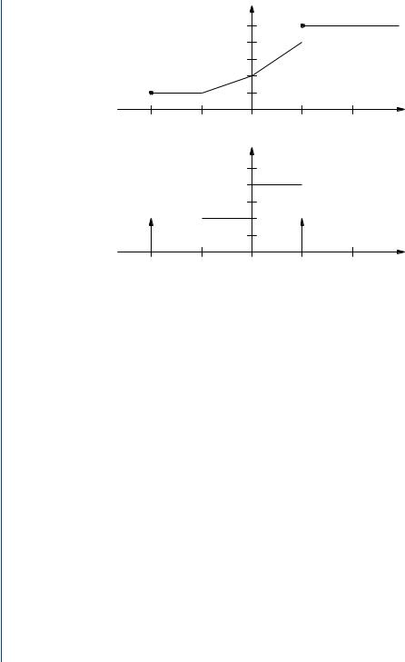
FIGURE 2.9: Cumulative distribution function and probability density function for Example 2.4.4

Example 2.4.4. Random variable x has CDF Fx given by

0,	α < −2
0.2,	−2 ≤ α < −1

Fx (α) = 0.2 + 0.2(α + 1), −1 ≤ α < 0

0.4 + 0.4α,	0 ≤ α < 1
1,	α ≥ 1.

Sketch Fx . Find and sketch the PDF fx .

Solution. Note that each piece of the given CDF is continuous. Examining the endpoints of each interval reveals that the CDF has discontinuities at α = −2 and at α = 1. The CDF and PDF are shown in Fig. 2.9. As is common practice, we have shown the Dirac delta functions as arrows with length corresponding to the area under the delta function. In addition, the weight (area) is shown next to each delta function. The PDF may be expressed as

fx (α) = 0.2δ(α + 2) + 0.2u(α + 1) + 0.2u(α) − 0.4u(α − 1) + 0.2δ(α − 1).

RANDOM VARIABLES 107

The CDF may be expressed as

Fx (α) = 0.2u(α + 2) + 0.2(α + 1)(u(α + 1) − u(α))

+ (0.2 + 0.4α)(u(α) − u(α − 1)) + 0.8u(α − 1).

The reader is encouraged to differentiate the above expression for Fx to obtain fx . It should be apparent that plotting the CDF and PDF significantly reduces the work involved.

Example 2.4.5. A coin is tossed n times. The probability of a head on any one toss is p and the probability of a tail is q , where p + q = 1. Let the RV x be the number of heads in n tosses. Find the CDF and the PDF for the RV x.

	Solution. The PMF for x is
		n	pk q n−k , α	=	k	=	0, 1, . . . , n
	px (α) =	k

0,

Consequently, the CDF is

N

Fx (α) =

k=0

and the PDF is

	otherwise.
n	pk q n−k u(α − k)
k

				n			n		pk q n−k δ(α − k).
Fx (α) =
				k=0			k
Drill Problem 2.4.1. The CDF of the RV x is given by
	0,				1				α < −2
		1		+				(α + 2), −2 ≤ α < 1
Fx (α) =	4				12
		1		+	1		(α		− 1), 1 ≤ α < 2
		2			4
Evaluate	1,								α ≥ 2.
								∞
			I1 =						α d Fx (α)
					−∞

and

∞

I2 = α2 d Fx (α).

−∞

Answers: 1/4, 17/6.

108 BASIC PROBABILITY THEORY FOR BIOMEDICAL ENGINEERS

Drill Problem 2.4.2. Evaluate the following integrals:

∞

I1 = ln(sin(π α)) d u(α − 0.3) ;

−∞

∞

I2 = sin(π α)(d u(α) + d u(α − 2));

−∞

∞

I3 = 2α d u(α + 3) ;

−∞

and

∞

I4 = 5u(t − 3) d u(t + 3) .

−∞

Answers: 0, −6, 0, −0.212.

Drill Problem 2.4.3. Evaluate the following integrals:

∞

I1 = ln(sin(π α))δ(α − 0.3) d α ;

−∞

∞

I2 = sin(π α)(δ(α) + δ(α − 2)) d α ;

−∞

∞

I3 = 2αδ(α + 3) d α ;

−∞

and

∞

I4 = 5u(t − 3)δ(t + 3) d t .

−∞

Answers: 0, −6, 0, −0.212.

Drill Problem 2.4.4. Two balls are selected at random from an urn that contains two blue, three red, and three green balls. Find the PDF for the random variable x, where x is the number of blue balls selected.

Answer: fx (α) =	1			3				15
		δ(α − 2)	+			δ(α − 1)	+		δ(α).
	28				7			28

RANDOM VARIABLES 109

2.5CONDITIONAL PROBABILITY

In Chapter 1, we discussed conditional probabilities. With events A and B defined on the probability space (S, F, P ), we defined the probability that event B occurs, given that event A occurred as

			P (B| A) =			P (A ∩ B)	.		(2.67)
						P (A)
Definition 2.5.1. Let x be a RV defined on (S, F, P ), and let B denote the event
			B = {ζ : x(ζ ) ≤ α}.
The conditional CDF for the RV x, given event A, is defined by
Fx| A(	α	| A) =	P (A ∩ B)	=	P ({ζ S : x(ζ ) ≤ α, ζ A})			.	(2.68)
			P (A)
							P (A)

If P (A) = 0 we define Fx| A to be any valid CDF.

If x is a discrete RV, we define the conditional PMF for the RV x, given event A, by

px| A(α| A) = Fx| A(α| A) − Fx| A(α−| A).					(2.69)
Similarly, if x is a continuous RV, we define the conditional PDF x, given event					A, by
fx| A(	α	| A) =	d Fx| A(α| A)	.	(2.70)
			d α

Note that the conditional CDF Fx| A is indeed a CDF in its own right; i.e., Fx| A is monotone nondecreasing, right-continuous, Fx| A(−∞| A) = 0, and Fx| A(∞| A) = 1.

If x is a discrete RV and P (A) = 0, from (2.69) we have
px| A(	α	| A) =	P (ζ S : x(ζ ) = α, ζ A)								,
									P (A)
so that
					px| A(α)				1
px| A(α| A) =								,	x−	({α}) A	(2.71)
						P (A)
				0,					otherwise.
Similarly, if x is a continuous RV and P (A) = 0, it follows from (2.70) that
						fx (α)			x−1({α}) A
fx| A(α| A) =							,				(2.72)
						P (A)
				0,					otherwise.

110 BASIC PROBABILITY THEORY FOR BIOMEDICAL ENGINEERS

Recall the discussion in Section 1.8 that a probability space (A, FA, PA) can be defined such that all conditional probabilities (given event A) on (S, F, P ) may be computed as unconditional probabilities on (A, FA, PA). Consequently, all remarks and properties regarding a CDF, PMF, and PDF are also valid for the corresponding conditional entities. On the probability space (A, FA, PA) we may define the RV y = x| A with CDF Fy (α) = Fx| A(α| A).

Example 2.5.1. Let the RV x have the PDF

1 − α, 0 < α < 1 fx (α) = α − 1, 1 < α < 2 0, otherwise.

Define the events A = {x > 1} and B = {0.5 < x < 1.5}. Find (a) Fx| A(α| A); (b) fx| A(α| A); and

(c) fx|B (α|B).

Solution

(a) By definition,

Fx| A(	α	| A) =	P (x ≤ α, x > 1)	=	P (1 < x ≤ α)	.
			P (A)
					P (x > 1)

Integrating the PDF from 1 to 2 we find that P (A) = P (x > 1) = 0.5, and

0, α < 1

Fx| A(α| A) = 2(Fx (α) − 0.5) = α2 − 2α + 1, 1 ≤ α < 2 1, α ≥ 2.

(b) Differentiating the result from (a) we obtain

0, α < 1

fx| A(α| A) = 2α − 2, 1 < α < 2 0, α > 2.

As an alternative, from (2.72) we obtain

fx| A	(α	| A	)	=	2 fx (α) = 2(α − 1), 1 < α < 2
					0,	otherwise.

(c)From the given PDF we find P (B) = P (0.5 < x < 1.5) = 0.25. Applying the definition of conditional CDF, we find

Fx|B (α|B) = P (0.5 < x < min{α, 1.5}) .

P (B)