Advanced Probability Theory for Biomedical Engineers - John D. Enderle

STANDARD PROBABILITY DISTRIBUTIONS 43

trick move also prevents him from ever getting pinned. The length of time it takes William to pin his opponent in each period of a wrestling match is given by:

period 1 : period 2 : period 3 :

fx (α) = 0.4598394 exp(−0.4598394α)u(α),

fx| A(α| A) = 0.2299197 exp(−0.2299197α)u(α), fx| A(α| A) = 0.1149599 exp(−0.1149599α)u(α),

where A = {Smith did not pin his opponent during the previous periods}. Assume each period is 2 min and the match is 3 periods. Determine the probability that William Smith: (a) pins his opponent during the first period: (b) pins his opponent during the second period: (c) pins his opponent during the third period: (d) wins the match.

58.Consider Problem 57. Find the probability that William Smith wins: (a) at least 4 of his first 5 matches, (b) more matches than he is expected to during a 10 match season.

59.The average time between power failures in a Coop utility is once every 1.4 years. Determine: (a) the probability that there will be at least one power failure during the coming year, (b) the probability that there will be at least two power failures during the coming year.

60.Consider Problem 59 statement. Assume that a power failure will last at least 24 h. Suppose Fargo Community Hospital has a backup emergency generator to provide auxilary power during a power failure. Moreover, the emergency generator has an expected time between failures of once every 200 h. What is the probability that the hospital will be without power during the next 24 h?

61.The queue for the cash register at a popular package store near Fargo Polytechnic Institute becomes quite long on Saturdays following football games. On the average, the queue is 6.3 people long. Each customer takes 4 min to check out. Determine: (a) your expected waiting time to make a purchase, (b) the probability that you will have less than four people in the queue ahead of you, (c) the probability that you will have more than five people in the queue ahead of you.

62.Outer Space Adventures, Inc. prints brochures describing their vacation packages as “Unique, Unexpected and Unexplained.” The vacations certainly live up to their advertisement. In fact, they are so unexpected that the length of the vacations is random, following an exponential distribution, having an average length of 6 months. Suppose that you have signed up for a vacation trip that starts at the end of this quarter. What is the probability that you will be back home in time for next fall quarter (that is, 9 months later)?

44ADVANCED PROBABILITY THEORY FOR BIOMEDICAL ENGINEERS

63.A certain brand of light bulbs has an average life-expectancy of 750 h. The failure rate of these light bulbs follows an exponential PDF. Seven-hundred and fifty of these bulbs were put in light fixtures in four rooms. The lights were turned on and left that way for a different length of time in each room as follows:

	ROOM	TIME BULBS LEFT ON, HOURS	NUMBER OF BULBS
	1	1000	125
	2	750	250
	3	500	150
	4	1500	225

After the specified length of time, the bulbs were taken from the fixtures and placed in a box. If a bulb is selected at random from the box, what is the probability that it is burnt out?

45

C H A P T E R 6

Transformations of Random Variables

Functions of random variables occur frequently in many applications of probability theory. For example, a full wave rectifier circuit produces an output that is the absolute value of the input. The input/output characteristics of many physical devices can be represented by a nonlinear memoryless transformation of the input.

The primary subjects of this chapter are methods for determining the probability distribution of a function of a random variable. We first evaluate the probability distribution of a function of one random variable using the CDF and then the PDF. Next, the probability distribution for a single random variable is determined from a function of two random variables using the CDF. Then, the joint probability distribution is found from a function of two random variables using the joint PDF and the CDF.

6.1UNIVARIATE CDF TECHNIQUE

This section introduces a method of computing the probability distribution of a function of a random variable using the CDF. We will refer to this method as the CDF technique. The CDF technique is applicable for all functions z = g (x), and for all types of continuous, discrete, and mixed random variables. Of course, we require that the function z : S → R , with z(ζ ) = g (x(ζ )), is a random variable on the probability space (S, , P ); consequently, we require z to be a measurable function on the measurable space (S, ) and P (z(ζ ) {−∞, +∞}) = 0.

The ease of use of the CDF technique depends critically on the functional form of g (x). To make the CDF technique easier to understand, we start the discussion of computing the probability distribution of z = g (x) with the simplest case, a continuous monotonic function g . (Recall that if g is a monotonic function then a one-to-one correspondence between g (x) and x exists.) Then, the difficulties associated with computing the probability distribution of z = g (x) are investigated when the restrictions on g (x) are relaxed.

6.1.1CDF Technique with Monotonic Functions

Consider the problem where the CDF Fx is known for the RV x, and we wish to find the CDF for random variable z = g (x). Proceeding from the definition of the CDF for z, we have for a

46 ADVANCED PROBABILITY THEORY FOR BIOMEDICAL ENGINEERS
monotonic increasing function g (x)
Fz(γ ) = P (z = g (x) ≤ γ ) = P (x ≤ g −1(γ )) = Fx (g −1(γ )),	(6.1)

where g −1(γ ) is the value of α for which g (α) = γ . As (6.1) indicates, the CDF of random variable z is written in terms of Fx (α), with the argument α replaced by g −1(γ ).

Similarly, if z = g (x) and g is monotone decreasing, then

Fz(γ ) = P (z = g (x) ≤ γ ) = P (x ≥ g −1(γ )) = 1 − Fx (g −1(γ )−).

(6.2)

The following example illustrates this technique.

Example 6.1.1. Random variable x is uniformly distributed in the interval 0 to 4. Find the CDF for random variable z = 2x + 1.

Solution. Since random variable x is uniformly distributed, the CDF of x is

0, α < 0 Fx (α) = α/4, 0 ≤ α < 4

1, 4 ≤ α.

Letting g (x) = 2x + 1, we see that g is monotone increasing and that g −1(γ ) = (γ − 1)/2. Applying (6.1), the CDF for z is given by

Fz(

) = Fx

γ 1

=

(

0,

(γ − 1)/2 < 0

4

2

− 1)

8

0 ≤ (

− 1)

2

γ

−

γ

/

,

γ

/

<

1,

4 ≤ (γ − 1)/2.

Simplifying, we obtain

0,

γ < 1

Fz(γ ) = (γ − 1)/8,

1 ≤ γ < 9

1,

9 ≤ γ ,

which is also a uniform distribution.

6.1.2CDF Technique with Arbitrary Functions

In general, the relationship between x and z can take on any form, including discontinuities. Additionally, the function does not have to be monotonic, more than one solution of z = g (x) can exist—resulting in a many-to-one mapping from x to z. In general, the only requirement on g is that z = g (x) be a random variable. In this general case, Fz(γ ) is no longer found by simple substitution. In fact, under these conditions it is impossible to write a general expression for Fz(γ ) using the CDF technique. However, this case is conceptually no more difficult than

TRANSFORMATIONS OF RANDOM VARIABLES 47

the previous case, and involves only careful book keeping. Let

A(γ ) = {x : g (x) ≤ γ }.	(6.3)
Note that A(γ ) = g −1((−∞, γ ]). Then
Fz(γ ) = P (g (x) ≤ γ ) = P (x A(γ )).	(6.4)
Partition A(γ ) into disjoint intervals { Ai (γ ) : i = 1, 2, . . .} so that
∞
A(γ ) = Ai (γ ).	(6.5)
i=1

Note that the intervals as well as the number of nonempty intervals depends on γ . Since the Ai ’s are disjoint,

Fz(γ ) =	∞
	P (x Ai (γ )).	(6.6)
	i=1

The above probabilities are easily found from the CDF Fx . If interval Ai (γ ) is of the form

Ai (γ ) = (ai (γ ), bi (γ )],	(6.7)
then
P (x Ai (γ )) = Fx (bi (γ )) − Fx (ai (γ )).	(6.8)
Similarly, if interval Ai (γ ) is of the form
Ai (γ ) = [ai (γ ), bi (γ )],	(6.9)
then
P (x Ai (γ )) = Fx (bi (γ )) − Fx (ai (γ )−).	(6.10)

The success of this method clearly depends on our ability to partition A(γ ) into disjoint intervals. Using this method, any function g and CDF Fx is amenable to a solution for Fz(γ ). The following examples illustrate various aspects of this technique.

Example 6.1.2. Random variable x has the CDF
0,	α < −1
Fx (α) = (3α − α3 + 2)/4,	−1 ≤ α < 1
1,	1 ≤ α.
Find the CDF for the RV z = x2.

48 ADVANCED PROBABILITY THEORY FOR BIOMEDICAL ENGINEERS

Solution. Letting g (x) = x2, we find

A

(γ )

= g

−1((

−∞

, γ ])

=

[−√

,

√

γ < 0

γ

,

γ

],

γ ≥ 0.

so that

Fz(γ ) = Fx (√γ ) − Fx ((−√γ )−).

Noting that Fx (α) is continuous and has the same functional form for −1 < α < 1, we obtain

0,					γ < 0
Fz(γ ) = (3√		− (√		)3)/2,	0 ≤ γ < 1
	γ		γ
1					1 ≤ γ .

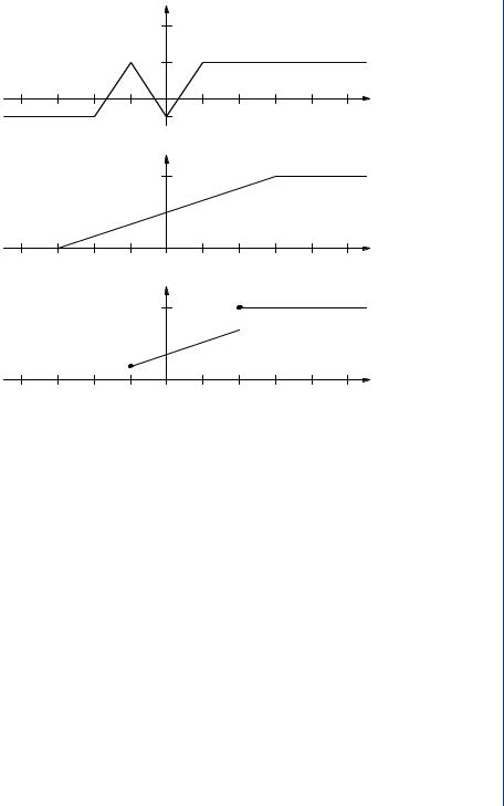
Example 6.1.3. Random variable x is uniformly distributed in the interval −3 to 3. Random variable z is defined by

−1,	x < −2
3x + 5,	−2 ≤ x < −1
z = g (x) = −3x − 1,	−1 ≤ x < 0
3x − 1,	0	≤ x < 1
2,	1	≤ x.

Find Fz(γ ).

Solution. Plots for this example are given in Figure 6.1. The CDF for random variable x is

0,	α < −3
Fx (α) = (α + 3)/6,	−3 ≤ α < 3
1,	3 ≤ α.

Let A(γ ) = g −1((−∞, ∞)). Referring to Figure 6.1 we find

γ − 5

,

γ < −1

A(

γ

) = −∞

,

−γ − 1

,

γ + 1

,

−1 ≤

γ <

2

3

3

3

R

2 ≤ γ .

Consequently,

0,

−γ − 1

−

γ < −1

Fz(

γ

) =

γ − 5

γ + 1

,

−1

γ <

2

Fx 3

+ Fx

− Fx

≤

3

3

1

2 ≤ γ .

TRANSFORMATIONS OF RANDOM VARIABLES 49

			g(x)
		4
		2
−3	−1	−1	1	3	x
			Fx (α)
		1
−3	−1		1	3	α
			Fz (γ )
		1
−3	−1		1	3	γ

FIGURE 6.1: Plots for Example 6.1.3.

Substituting, we obtain

0,

γ < −1

Fz(

γ

) =

1

γ − 5

+ 3 +

γ + 1

−

−γ − 1

=

γ + 2

,

−1 ≤

γ <

2

6

3

3

6

3

1

2 ≤ γ .

Note that Fz(γ ) has jumps at γ = −1 and at γ = 2.

Whenever random variable x is continuous and g (x) is constant over some interval or intervals, then random variable z can be continuous, discrete or mixed, dependent on the CDF for random variable x. As presented in the previous example, random variable z is mixed due to the constant value of g (x) in the intervals −3 ≤ x < −2 and 1 ≤ x < 3. In fact, z is a mixed random variable whenever g (α) is constant in an interval where fx (α) = 0. This results in a jump in Fz and an impulse function in fz. Moreover, z = g (x) is a discrete random variable if g (α) changes values only on intervals where fx (α) = 0. Random variable z is continuous if x is continuous and g (x) is not equal to a constant over any interval where fx (α) = 0.

50 ADVANCED PROBABILITY THEORY FOR BIOMEDICAL ENGINEERS

Example 6.1.4. Random variable x has the PDF

fx	(α)	=	(1 + α2)/6,	−1 < α < 2
			0,	otherwise.

Find the PDF of random variable z defined by

x − 1,	x ≤ 0
z = g (x) = 0,	0 < x ≤ 0.5
1,	0.5 < x.

Solution. To find fz, we evaluate Fz first, then differentiate this result. The CDF for random variable x is

0,

α < −1

Fx (α) = (α3 + 3α + 4)/18, −1 ≤ α < 2

1,

2 ≤ α.

Figure 6.2 shows a plot of g (x). With the aid of Figure 6.2, we find

(−∞, γ + 1],

γ ≤ −1

A

(γ )

= {x

:

(

)

≤

γ

} =

(−∞, 0],

,

−1 ≤ γ < 0

g x

,

0

.

5]

0 ≤

γ <

1

(−∞

(−∞, ∞),

1 ≤ γ .

Consequently,

Fx (γ + 1),

γ ≤ −1

Fz

(γ )

=

Fx (0),

,

−1 ≤ γ < 0

Fx (0

.

5)

0 ≤

γ <

1

1,

1 ≤ γ .

	g( x )
	1
−1	1	2	x
	−1
	−2

FIGURE 6.2: Transformation for Example 6.1.4.

	TRANSFORMATIONS OF RANDOM VARIABLES 51
Substituting,
	0,	γ < −2
Fz(γ ) =	((γ + 1)3 + 3γ + 7)/18,	−2 ≤ γ < −1
	2/9,	−1 ≤ γ < 0
	5/16,	0 ≤ γ < 1
	1,	1 ≤ γ .

Note that Fz(γ ) has jumps at γ = 0 and γ = 1 of heights 13/144 and 11/16, respectively. Differentiating Fz,

fz(

γ

) =

3γ 2 + 6γ + 6

(u(

γ

+ 2) − u(

γ

+ 1)) +

13

δ

γ

) +

11

δ

γ

− 1)

.

18

144

16

(

(

Example 6.1.5. Random variable x is uniformly distributed in the interval from 0 to 10. Find the CDF for random variable z = g (x) = − ln(x).

Solution. The CDF for x is
0,	α < 0
Fx (α) = α/10,	0 ≤ α < 10
1,	10 ≤ α.
For γ > 0, we find

A(γ ) = {x : − ln(x) ≤ γ } = (e −γ , ∞),

so that Fz(γ ) = 1 − Fx ((e −γ )−). Note that P (x ≤ 0) = 0, as required since g (x) = − ln(x) is not defined (or at least not real–valued) for x ≤ 0. We find

Fz(γ ) =	0,	γ < ln(0.1)
	1 − e −0.1γ ,	ln(0.1) ≤ γ .

The previous examples illustrated evaluating the probability distribution of a function of a continuous random variable using the CDF technique. This technique is applicable for all functions z = g (x), continuous and discontinuous. Additionally, the CDF technique is applicable if random variable x is mixed or discrete. For mixed random variables, the CDF technique is used without any changes or modifications as shown in the next example.

Example 6.1.6. Random variable x has PDF

fx (α) = 0.5(u(α) − u(α − 1)) + 0.5δ(α − 0.5).

Find the CDF for z = g (x) = 1/x2.

52 ADVANCED PROBABILITY THEORY FOR BIOMEDICAL ENGINEERS

Solution. The mixed random variable x has CDF

0,

α < 0

Fx

(α)

=

.

0.5α,

α,

0 ≤ α < 0.5

5 + 0

.

0

.

5 ≤

α <

1

0

5

1,

1 ≤ α.

For γ < 0, Fz(γ ) = 0. For γ > 0,

1

1

A(γ ) = {x : x−2 ≤ γ } = −∞, − √

√

, ∞ ,

γ

γ

so that

Fz(γ ) = Fx (−1/√γ ) + 1 − Fx ((1/√γ )−).

Since Fx (−1/√γ ) = 0 for all real γ , we have

0,

(1/√

)−

< 0

γ

0.5γ −1/2,

0 ≤ (1/√

)− < 0.5

Fz

(γ )

=

1

−

γ

0.5 + 0.5γ −1/2,

0.5 ≤ (1/√

)− < 1

γ

1,

1

≤

(1/√γ )−.

After some algebra,

0,

γ < 1

Fz(γ ) = 0.5 − 0.5γ −1/2, 1 ≤ γ < 4

1

−

0.5γ −1/2

,

4

≤

γ .

Drill Problem 6.1.1. Random variable x is uniformly distributed in the interval −1 to 4. Random variable z = 3x + 2. Determine: (a) Fz(0), (b)Fz(1), (c ) fz(0), (c ) fz(15).

Answers: 0, 2/15, 1/15, 1/15.

Drill Problem 6.1.2. Random variable x has the PDF

fx (α) = 0.5α(u(α) − u(α − 2)).

Random variable z is defined by
−1,	x < 1
z = x,	−1	≤ x ≤ 1
1,	x	> 1.

Determine: (a) Fz(−1/2), (b)Fz(1/2), (c )Fz(3/2), (d ) fz(1/2).

Answers: 0, 1, 1/16, 1/4.