Downloads / holland_2000

The MIT Press Journals

http://mitpress.mit.edu/journals

This article is provided courtesy of The MIT Press.

To join an e-mail alert list and receive the latest news on our publications, please visit: http://mitpress.mit.edu/e-mail

Building Blocks, Cohort Genetic Algorithms,

and Hyperplane-Defined Functions

John H. Holland

Professor of Psychology

Professor of Computer Science and Engineering

The University of Michigan

Ann Arbor, MI 48109, USA

and

External Professor

Santa Fe Institute

Santa Fe, NM 87501, USA

Abstract

Building blocks are a ubiquitous feature at all levels of human understanding, from perception through science and innovation. Genetic algorithms are designed to exploit this prevalence. A new, more robust class of genetic algorithms, cohort genetic algorithms (cGA’s), provides substantial advantages in exploring search spaces for building blocks while exploiting building blocks already found. To test these capabilities, a new, general class of test functions, the hyperplane-defined functions (hdf’s), has been designed. Hdf’s offer the means of tracing the origin of each advance in performance; at the same time hdf’s are resistant to reverse engineering, so that algorithms cannot be designed to take advantage of the characteristics of particular examples.

Keywords

Building blocks, chromosome-like strings, crossover, fitness, genetic algorithms, schema, search spaces, robustness, selection, test functions.

1 Introduction

The “building block thesis” holds that most of what we know about the world pivots on descriptions and mechanisms constructed from elementary building blocks. My first comments on this thesis, though it did not yet have that name, were published at the 1960 Western Joint Computer Conference1 (WJCC) as part of a special session on “The design, programming, and sociological implications of microelectronics” (Holland, 1960). The paper ended by tying together topics that play a key role in the thesis: implicit definition of structure, connected generators, hierarchical definition, adaptation, autocatalytic systems, Art Samuel’s checkersplayer, and implicit definition of the problem space (as contrasted to a state-by-state definition). In both the session and the published proceedings, my paper was followed by Al Newell’s wonderful riff on the framework I’d presented, a paper still exciting to read after all these years. The upshot was an avid desire, on my part, to look further into algorithmic approaches to adaptation.

1As an aside, the WJCC was a remnant of an east-coast/west-coast division in the computing community, a rift that had largely healed by 1960, but similar at its height to the current division in the EC community. None of the exploration reported there would likely be considered “computer science” under today’s hardened definitions, but far-horizon exploration was encouraged in those days.

c 2000 by the Massachusetts Institute of Technology

Evolutionary Computation 8(4): 373-391

J. Holland

Level (science)	Typical Mechanisms
Nucleus (physics)	quarks, gluons
Atom (physics)	protons, neutrons, electrons
Gas & Fluid (physics)
con ned (e.g., a boiler)	PVT laws, ows
free (e.g., weather)	circulation (e.g. fronts), turbulence
Molecule (chemistry)	bonds, active sites, mass action
Organelle (microbiology)	enzymes, membranes, transport
Cell (biology)	mitosis, meiosis, genetic operators
Organism (biology)	growth factors, apoptosis, other mor-
	phogenetic operators
Ecosystem (ecology)	predation, symbiosis, mimicry

Building blocks from lower levels provide constraints and suggest what to look for at higher levels. Proposed additions at any level must be consistent with observations at all levels.

Figure 1: A typical set of interlocked levels of investigation in science.

The building block thesis has been validated repeatedly in the scientific advances of the 40 years since that WJCC. Each major advance over this period, as was also the case in earlier years, depended on the discovery and recombination of well-chosen building blocks. Section 2 of this paper presents enough old and new examples to make this claim plausible. Once a computer scientist starts thinking about building blocks as a source of innovation, the next obvious step is to look for algorithms that can discover and exploit building blocks. It is my claim that genetic algorithms (GA’s) are particularly qualified for this task. Sections 3 and 4 present a part of that argument, while Section 5 outlines some of the obstacles that stand in the way of unfettered use of GA’s for this purpose. Section 6 discusses a new class of GA’s, called cohort GA’s (cGA’s), designed to overcome these obstacles, while Section 7 outlines a broad class of test functions, the hyperplane defined functions (hdf’s), that allow one to trace in detail just how the obstacles are overcome. Section 8 discusses cGA/hdf interaction, and Section 9 makes some observations about this interaction. The paper closes with a look to the future.

2 Building Blocks

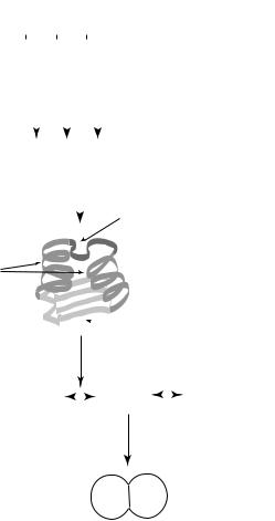
The successive levels of building blocks used in physics are familiar to anyone interested in science — nucleons constructed from quarks, nuclei constructed from nucleons, atoms constructed from nuclei, molecules constructed from atoms, and so on (see Figure 1). Nowadays a similar succession presents itself in daily newspaper articles discussing progress in biology: chromosomal DNA constructed from 4 nucleotide building blocks; the basic structural components of enzymes: alpha helices, beta sheets, and the like, constructed from 20 amino acids; standard “signaling” proteins for turning genes “on” and “off,” and “autocatalytic bio-circuits,” such as the citric acid cycle, that perform similar functions over extraordinarily wide ranges of species; organelles constructed from situated bio-circuits, and so on (see Figure 2). And, of course, there are the long-standing taxonomic categories: species, genus, family, etc., specified in terms of morphological and chromosomal building blocks held in common. However, the pervasiveness of building blocks only becomes

374	Evolutionary Computation Volume 8, Number 4

Cohort GAs and Hyperplane-Defined Functions

LEVELS

DNA sequence (Chromosome)

GAATCAAGC ... ... CGAC ...

4 generators (building blocks)

<A, G, C, T>

transcription

(triplet code)

Amino acid sequence

~20 generators

glu - ser - ser - ...

<arganine, glutamine, ... >

folding

active site

Protein (enzyme, etc.) structural generators <a-helix, b-sheet, ... >

a - helices

b - sheet

catalysis

Bio-circuits	U + V		W + X		Y + Z
<citric acid cycle, ... >

behavior ("reservoir filling")

Fitness

< "reservoirs", niche space, ... >

A metazoan typically has dozens of alleles that distinguish it from other organisms of its species. These differences are not fitness-neutral.

Most recombinations yield a change in fitness.

[Emergence conjecture: Neutrality decreases with each successive level.]

Figure 2: Levels and building blocks in biological systems.

Evolutionary Computation Volume 8, Number 4

375

J. Holland

apparent when we start looking at other areas of human endeavor. In some cases we take building blocks so much for granted that we’re not even aware of them. Human perception is a case in point. The objects we recognize in the world are always defined in terms of elementary, reusable building blocks, be they trees (leaves, branches, trunks,...), horses (legs, body, neck, head, blunt teeth,...), speech (a limited set of basic sounds called phonemes), or written language (the 26 letters of English, for example).

In other cases we just don’t make the building blocks explicit. Consider two major inventions of the 20th century, the internal combustion engine and the electronic computer. The building blocks of the internal combustion engine: gears, Venturi’s aspirator, Galvani’s sparking device, and so on, were well-known prior to the invention. The invention consisted in combining them in a new way. Similarly, the components of early electronic programmable computers: wires, Geiger’s counting device, cathode ray tubes, and the like, were well-known. Even earlier, Babbage had spelled out an overall architecture using long-standard, mechanical building blocks (gears, ratchets, levers, etc.). The later invention consisted in combining the electronic building blocks in a way that implemented Babbage’s mechanical layout. And, of course, building blocks underpin the critical step for universal computation: arbitrary algorithms are constructed by combining copies of a small set of basic instructions. For both the internal combustion engine and the programmable computer, the building blocks were a necessary precursor, but the innovation required a new combination of the blocks. That is a theme to which we’ll return.

There are two main characteristics of building blocks: (i) they must be easy to identify (once they’ve been discovered or picked out), and (ii) they must be readily recombined to form a wide variety of structures (much as can be done with children’s building blocks). Descriptions so-constructed will only be useful if there are many, frequently encountered objects that can be so described. For actual constructions, as contrasted to descriptions, building blocks will only be useful if there are many objects (useful and not so useful) that can be constructed from the blocks.

3 Toward Genetic Algorithms

Building blocks play a central role both in Darwin’s original formulation of natural selection and in the neo-Darwinian synthesis. This role becomes quite clear when we consider Darwin’s strong emphasis on the relation between artificial selection (breeding) and natural selection:

Artificial selection depends upon mating animals or plants that have desirable characteristics. That is, the breeder mates individuals that have different, recognizable building blocks (be it long legs or an unusual color) that contribute to capabilities the breeder desires. After mating, the breeder artificially selects the best of the offspring, those combining more of the desired characters in a single individual, for further breeding. The common term for this kind of breeding is “crossing.” We now know that, at the chromosomal level, “crossover” (crossing over of the relevant chromosomes) implements “crossing,” although artificial selection was practiced for millennia prior to this understanding. Natural selection operates in a similar fashion, but now the favored characteristics are those leading to the acquisition of resources that can be turned into offspring.

[It used to be a common assumption that, at the level of the genome, building blocks are specified by individual genes having cumulative additive effects. Much of the early seminal work, including Fisher’s (1930) fundamental mathematical development, takes this

376	Evolutionary Computation Volume 8, Number 4

Cohort GAs and Hyperplane-Defined Functions

assumption as a starting point. However, it is now amply clear from work in genomics and proteonomics, that (i) linked groups of genes can serve as building blocks under crossover and (ii) the interactions they encode can be highly nonlinear. See for example, Schwab and Pienta (1997), Hutter et al. (2000), Walter et al. (2000), Lander and Weinberg (2000), and Rubin et al. (2000).

Typically, in both artificial and natural selection, there are large sets of possibilities to be explored. These sets are often called search spaces. In the simplest form, each element (possibility) in a search space has an assigned value called its fitness. In artificial selection, this fitness measures the extent to which an element (individual) has the characteristics desired by the breeder. In natural selection, the fitness measures the ability of the corresponding individual to find and convert resources into offspring.2

In exploring this search space, the usual objective is not so much one of finding the best individual, as it is to locate a succession of improvements. The search is for individuals of ever-higher fitness. Such a search could be implemented as a uniform random sampling, and there are search spaces for which it can be shown that there is no faster search technique. However, this is not a good way to explore a search space that has relevant regularities. If the regularities can be exploited to guide the search, search time can be reduced by orders of magnitude. Building blocks supply regularities that can be exploited.

It is clear that both artificial and natural selection can locate individuals of increasing fitness in quite complex search spaces. Current work in molecular biology makes it increasingly clear that these “solutions” depend on new combinations of extant building blocks, along with the occasional discovery of a new building block. We only need to look again to Darwin to see that these ideas played a prominent role in his treatises. For example, Darwin’s discussion of the origin of complex adaptations, such as the eye, pivots on the accumulation and exploitation of appropriately simple components that were already valuable in other contexts.

4 Designing Genetic Algorithms

It is not much of a leap, then, to think of adopting a Darwinian approach to exploring search spaces that abound in building blocks. Indeed, given the pervasiveness of building blocks in the actual and figurative devices we use to understand the world, this would seem a productive way to approach many of the world’s complexities. The question then becomes:

How do we turn Darwin’s ideas into algorithms?

With our knowledge of chromosomes as the carriers of heredity, it seems reasonable to start by encoding individuals in the search space as chromosome-like strings. Binary encodings work, though more complex encodings have been used. Once we have a string representation it is then natural to want to relate building blocks to pieces of strings. This is now familiar ground, though it took some thought at the outset.

Given a set S containing all objects of interest, it is common in mathematics to identify a property of an object with the subset of all objects that have the property. There is a set of easily defined subsets of S that makes a good starting point. Treat each string position (locus) as a dimension of the space S and then consider the hyperplanes in S. For the set

2I will not discuss here the shortcomings of such one-dimensional measures, nor will I discuss the advantages of an implicit definition of fitness over this explicit definition.

Evolutionary Computation Volume 8, Number 4

377

J. Holland

S of binary strings of length n, f1; 0gn , the set of all hyperplanes H can be identified with the set f1; 0; #gn. The string s 2 S belongs to hyperplane h 2 H if and only if each of the non-# bits in the string h matches the corresponding bit in the string s. That is, the strings h and s match at all positions where there is not a #. Accordingly, the string h = 1#0# # specifies the hyperplane consisting of all strings in S that start with a 1 and have a 0 at the third position. These hyperplanes are called schemata in papers dealing with genetic algorithms.

From the point of view of genetics, all the individuals belonging to a given hyperplane hold certain alleles in common. If this set of alleles is correlated with some increment in fitness, the set constitutes a useful building block called a coadapted set of alleles. If we were talking of cars instead chromosomes, we might be considering the advantages of a coadapted set of components called a fuel injection system.

How can an algorithm discover and exploit hyperplanes corresponding to coadapted sets of alleles? This is not the place to review the standard implementations of genetic algorithms. Most reading this paper will be familiar with GA’s; for those not so informed, Melanie Mitchell’s (1996) book is an excellent introduction. Suffice it to say that a typical GA operates on a population (set) B of n strings by iterating a three-step procedure:

1.Evaluate the fitness f(s) in the search space of each s 2 B.

2.Select n=2 pairs of strings from B, biased so that strings with higher fitness are more likely to be chosen.

3.Apply genetic operators, typically crossover and mutation, to the pairs to generate n=2 new pairs, replacing the strings in B with the n new strings so created; return to step

(1).

It takes a theorem, a generalization of Fisher’s famous Fundamental Theorem, to show that this simple procedure does interesting things to building blocks. Let f^h be the average observed fitness of the strings in B (if any) that belong to schema h, and let f^ be the average fitness of all the strings in B. Further, let the bias for selecting a given string in step (2) above be f^h=f^. Then it can be shown that the expected proportion of instances of h in the population formed in step (3) is bounded below by

^ ^	, eh)Ph
(fh=f)(1

where Ph is the proportion of strings in population B belonging to h, and the “error function” eh measures the destruction of instances of h by the genetic operators. eh is an invariant property of h — for example, eh increases with the distance between the endpoints of the defining loci for the schema h. This theorem is called the schema theorem (Holland, 1992).

In intuitive terms, this theorem says that the number of instances of a building block increases (decreases) when the observed average fitness in the current generation B is above (below) the observed population average. The theorem holds for all schemata represented in the population. In typical cases, eh is small for “short” schemata (say, schemata for which the distance between endpoints is less than a tenth the length of the string). For such schemata the error term can be ignored so that the number of instances of the schema in the next generation increases (decreases) when f^h=f^ > 1 (f^h=f^ < 1). For realistic values

378	Evolutionary Computation Volume 8, Number 4

Cohort GAs and Hyperplane-Defined Functions

of population size n and strings of any considerable length, say length > 100, it is easy to show that the number of schemata so processed vastly exceeds n. That is, the number of schemata manipulated as if the statistic f^h=f^ had been calculated is much larger than the number of strings explicitly processed. This is called implicit parallelism (Holland, 1992).

[In recent years, there have been glib, sometimes blatantly incorrect, statements about the schema theorem. One widely distributed quote claimed that the theorem was “either a tautology or incorrect.” It is neither. It has been carefully reproved in the context of mathematical genetics (Christiansen and Feldman, 1998), and it is no more a tautology than Fisher’s theorem. Quite recently a book purporting to provide the mathematical foundations for the “simple genetic algorithm (SGA)” says “. . . the ‘schema theorem’ explains virtually nothing about SGA behavior” (Vose, 1999, xi). Even explanations as brief as the one above make it clear that the theorem provides insight into the generation-to-generation dynamics of coadapted sets of alleles, as does Fisher’s theorem with respect to individual alleles. That same book offers, as its own explanation of dynamics, stochastic vectors wherein, for small populations and short strings, the largest entry — the most probable population — can be smaller than the reciprocal of the number of atoms in the universe! Standard mathematical approaches, such as Markov processes and statistical mechanics, typically offer little insight into the dynamics of processes that involve the nonlinearities inherent in coadaptations.]

It is clear from the schema theorem that a GA does exploit building blocks on a generation-by-generation basis. Crossover shows up in the schema theorem only as an impediment (usually slight) that increases eh. What purpose does crossover serve then? As is well-known to most practitioners, it serves two purposes: First of all, it recombines building blocks, bringing blocks residing on separate strings into combination on a single string. The second effect is more subtle. Crossover uncovers new building blocks by placing alleles in new contexts. Moreover, as we’ve seen in Section 2, building blocks are often combinations of more elementary building blocks, so recombination works at this level, too.

It’s worth a moment to put these observations in the broader context of biology. It is well-known that the crossover rate in mammals is about 6 orders of magnitude greater than the point mutation rate. Four main explanations have been given for the prevalence of crossover:

i.Crossover provides long (random) jumps in the space of possibilities, thus providing a way off of local maxima.

ii.Crossover repairs mutational damage by sequestering deleterious mutations in some offspring while leaving other offspring free of them.

iii.Crossover provides persistent variation that enables organisms to escape adaptive targeting by viruses, bacteria, and parasites.

iv.Crossover recombines building blocks.

I’ve listed these explanations in what I consider to be their order of (increasing) importance. All four explanations have some basis in experiment and observation but, given the overwhelming use of building blocks at all biological levels, it would seem that (iv) is sufficient in itself to account for the prevalence of crossover.

Evolutionary Computation Volume 8, Number 4

379

J. Holland

5 Robustness

Are GA’s, then, a robust approach to all problems in which building blocks play a key role? By no means! After years of investigation we still have only limited information about the GA’s capabilities for exploiting building blocks. In an attempt to learn more of the GA’s capabilities along these lines, several of us defined a class of building-block-based functions some years ago. We called them Royal Road (RR) functions (Mitchell et al., 1992) because improvement in the RR domain depended entirely on the discovery and exploitation of building blocks. We even thought that a GA would easily “outrun” competitors on this royal road.

We were wrong on several counts. First of all, in trying to make the functions simple, we made them too simple. The RR functions are convex, thus constituting a single “hill” to be climbed. There are gradient algorithms that, once positioned at the base of a hill, can double the accuracy of the “hilltop” coordinates with every iteration. No GA can move that fast. Worse yet, there are mutation-only algorithms that perform quite competitively in convex domains. Lesson 1: If you want test functions that exhibit the GA’s strength, don’t use convex functions.

There was a second flaw in the particular RR functions we used in our tests. They were too shallow. In the RR functions, building blocks at each level are formed from two adjacent building blocks at the previous level. As a result, building blocks at the next- to-highest level occupy half the chromosome, and they have a 50-50 probability of being “destroyed” each time crossover occurs. Because we used four-level functions, the GA had substantial difficulty getting beyond the first two levels. We call this “the saturation effect.” Because the GA’s greatest strengths lie in finding improvements, not in optimization, shallow functions are not a good test of performance. Lesson 2: If you want test functions that exhibit the GA’s strengths, use “deep” functions.

There was a third, more subtle difficulty, only partially attributable to the RR functions, though they highlighted the problem. It is a problem called “hitchhiking,” a phenomenon well-known in population genetics, but previously little studied in the context of GA’s. Hitchhiking occurs when some newly discovered allele (or coadapted set of alleles) offers great fitness advantages (say, DDT resistance for an insect species immersed in a DDT-rich environment). Then, as that allele spreads rapidly through the population, so do nearby, closely linked alleles (though they may make no contribution to the fitness). The net result is a greatly reduced exploration of alternatives at the loci involved in hitchhiking.

The hitchhiking problem presents typical GA’s with a dilemma. One side of the dilemma occurs when the scaled maximum reproduction rate is set high to provide rapid increase in above-average schemata. Then the defining bits of the schemata in the best string(s) in the population, along with the nearby bits, quickly come to occupy most of the population. That is, the nearby bits “hitchhike” to a prominence in the population, leaving few variants at those loci. This loss of diversity in the vicinity of the better schemata greatly impedes the search for further improvements. The effect is particularly damaging in a smaller population. Consider a population of 1000 individuals and a newly discovered individual with a scaled fitness of 2 (i.e., the individual produces 2 offspring for the next generation). If successive progeny of that individual retain a similarly high scaled fitness, the schemata in that individual, and nearby bits, will appear in almost every individual in the population in 10 generations. In such a short time, genetic operators like mutation cannot introduce enough differences into the population to counteract this rapid loss of diversity.

380	Evolutionary Computation Volume 8, Number 4

Cohort GAs and Hyperplane-Defined Functions

The other side of the dilemma arises if the reproduction rate for the best string is scaled downward to 1.2 or less, to give the GA time to counteract hitchhiking. Then we encounter difficulties because of the way in which typical GA’s handle “fractional offspring.” Almost all GA’s use some variant of a stochastic approach to deal with the fractional part of the fitness: For fitness 1.2, for example, a second offspring is produced with probability 0.2. Under this approach, the expected number of offspring for this individual, after several generations, is correct. We would expect to find 2 copies of an individual of fitness 1.2 after 4 generations (1:24 = 2). However, the variance associated with this expectation is large; the probability of only one copy after 4 generations is 0.4. Valuable schemata are likely to be lost under such circumstances.

This dilemma motivates a new class of genetic algorithms which I will discuss in the next section. The two earlier problems, convexity and shallowness, motivate a new class of test functions which I will discuss in Section 7.

6 Cohort Genetic Algorithms

Cohort genetic algorithms (cGA’s) are designed to allow low maximal reproduction rates without suffering the high variance induced by a stochastic approach to fractional offspring. The central idea for the cGA is that a string’s fitness determines how long it will have to wait before it produces offspring. A string of high fitness produces offspring quickly, while a string of low fitness may have to wait a long time before reproducing. With this arrangement, all strings can have the same number of offspring, say two, at the time they reproduce. The difference lies in the interval that must elapse before the two offspring are produced. Clearly, a highly fit string with building blocks that yield highly fit offspring will, over multi-generational time T, have many more progeny than a string of lower fitness. A little calculation shows that the variance of this method of reproduction is much less than the variance under the probabilistic approach to fractional offspring.

To implement this delayed-reproduction idea, the population of the cGA is divided into an ordered set of non-overlapping subpopulations called cohorts. Reproduction is carried out by cycling through the cohorts in the given order, determining the offspring for individuals in cohort 1, then cohort 2, and so on. When the last cohort is reached, the procedure returns to cohort 1 and is repeated.

Reproduction in cohort i, in a simple cGA with N cohorts, proceeds at follows:

1.Each string in cohort i produces 2 offspring.

2.The fitness u of each offspring is determined and is scaled using a function f(u), where f(u) = 1:2, say, for the maximum fitness so far observed, and f(u) = 1 for the current average fitness.

3.The doubling time d(u) corresponding to fitness f(u) is used to place each offspring in cohort (i + d(u)) mod N. [The doubling time for f(u) < 1:2 is roughly d(u) = :8=(f(u) , 1). When (f(u) , 1) < :25, say, it is pragmatically useful to use a linear function of f(u) , 1, taking arguments :25 > x > ,1, to distribute the corresponding offspring over the cohorts that lie between 16 and N steps “ahead” of the current cohort. Note that this provision assigns cohorts to offspring that are below average, whereas strict use of doubling time would put them in an infinitely distant cohort.]

Evolutionary Computation Volume 8, Number 4

381