Chen The electron capture detector

REFERENCES 137

69.Dressler, R.; Allan, M.; and Haselbach, E. Chemia 1985, 39, 385.

70.Fenzlaff, H. and Illenberger, E. Int. J. Mass Spectrom. Ion Phys. 1984, 32, 185.

71.Spyrou, S. M. and Christophorou, L. G. J. Chem. Phys. 1985, 82, 1048.

72.Wentworth, W. E.; Limero, T.; and Chen, E. C. M. J. Phys. Chem. 1987, 91, 241.

73.Klots, C. E.; Compton, R. N.; and Raaen, V. F. J. Chem. Phys. 1974, 60, 1177.

74.Hiraoka, K.; Mizuno, T.; Eguchi, D.; Takao, K.; Iino, T.; and Yamabe, S. J. Chem. Phys. 2002, 116, 7574.

75.Miller, T. M.; Morris, R. A.; Miller, A. E. S.; Viggiano, A. A.; and Paulson, J. F. Int. J. Mass Spectrom. Ion Proc. 1994, 135, 195.

76.Dillow, G. W. and Kebarle, P. J. Amer. Chem. Soc. 1989, 111, 5592.

77.Chen, E. S. D.; Chen, E. C. M.; Sane, N.; and Shultze, S. Bioelectrochem. Bioenerget. 1999, 48, 69.

78.Chen, E. C. M. and Wentworth, W. E. J. Chem. Phys. 1975, 63, 3183.

79.Streitweiser, A. S. Molecular Orbital Theory for Organic Chemists. New York: Wiley,

1961, pp. 159–172.

80.Dirac, P. Proc. Roy. Soc. Lond. 1929, A123, 714.

81.Lesk, A. M. Phys. Rev. 1968, 171, 7.

82.Hylleras, E. Z. Phys. 1930, 60, 624.

83.Pekeris, C. L. Phys. Rev. 1962, 126, 1470.

84.Lykke, K. R.; Murray, K. K.; and Lineberger, W. C. Phys. Rev. A 1991, 43, 6104.

85.Weis, A. Phys. Rev. 1961, 122, 1826.

86.Clementi, E. Phys. Rev. 1964, 135, A980.

87.Curtis, L. A.; Redfern, P. C.; Raghavachari, K.; and Pople, J. A. J. Chem. Phys. 1998, 109, 42.

88.Younkin, J. M.; Smith, L. J.; and Compton, R. N. Theoret. Chem. Acta 1976, 41, 157.

89.Dewar, M. J. S.; Hashmall, J. A.; and Trinajatic. J. Amer. Chem. Soc. 1970, 92, 5555.

90.Dewar, M. J. S. and Rzepa, H. S. J. Amer. Chem. Soc. 1978, 100, 784.

91.Huh, C.; Kang, C. H.; Lee, H. W.; Nakamura, H.; Mishima, M.; Tsuno,Y.; and Yamataka,

H.Bull. Chem. Soc. Japan 1999, 72, 1083.

92.Lee, T. J. J. Phys. Chem. 1963, 76, 360.

93.Mahan, B. H. J. Chem. Phys. 1966, 44, 2182.

94.Chen, E. C. M.; George, R. D.; and Wentworth, W. E. J. Chem. Phys. 1968, 49, 1973.

95.Fehsenfeld, F. C. J. Chem. Phys. 1970, 53, 2000.

96.Fessenden, R. W. and Bansal, K. M. J. Chem. Phys. 1970, 53, 3468.

97.Mothes, K. G. and Schindler. Ber. Bunsenges Phys. Chem. 1971, 75, 936.

98.Davis, F. J.; Compton, R. N.; and Nelson, D. R. J. Chem. Phys. 1973, 59, 2324.

99.Gant, K. S. and Christophorou, L. G. J. Chem. Phys. 1976, 65, 2977.

100.Hildebrandt, G. F.; Kellert, F. G.; Dunning, F. B.; Smith, K. A.; and Stebbings, R. F.

J.Chem. Phys. 1978, 68, 1349.

101.Crompton, R. W. and Haddad, G. N. Aust. J. Phys. 1983, 36, 15.

102.Spyrou, S. M. and Christophorou, L. G. J. Chem. Phys. 1985, 82, 1048.

138COMPLEMENTARY EXPERIMENTAL AND THEORETICAL PROCEDURES

103.Adams, N. G.; Smith, D.; Alge, E.; and Burdon, J. Chem. Phys. Lett. 1985, 116, 460.

104.Chutjian, A. and Alajajian, S. H. J. Phys. B 1985, 18, 4159.

105.Wentworth, W. E.; Limero, T.; and Chen, E. C. M. J. Phys. Chem. 1987, 91, 241.

106.Shimamori, H.; Tatsumi, Y.; Ogawa, Y.; and Sunagawa, T. J. Chem. Phys. 1992, 97, 6335.

107.Shimamori, H.; Tatsumi, Y.; and Sunagawa, T. J. Chem. Phys. 1993, 99, 7787.

108.Miller, T. M.; Miller, S.; and Paulson, J. F. J. Chem. Phys. 1994, 100 8841.

109.Smith, D. and Spanel, P. I. Adv. At. Mol. Opt. Phys. 1994, 32, 307.

110.Matejcik, S.; Mark, T. D.; Spanel, P.; Smith, D.; Jaffke, T.; and Illenberger, E. J. Chem. Phys. 1995, 102, 2516.

111.Vogt, D.; Hauffe, B.; and Neuert, H. Z. Phys. 1970, 232, 439.

112.Bailey, T. L. and Mahadevan, P. J. Chem. Phys. 1970, 52, 179.

113.Stockdale, J. A. D.; Compton, R. N.; Hurst, G. S.; and Reinhardt, P. W. J. Chem. Phys. 1969, 50, 2176.

114.D’sa, E. D.; Wentworth, W. E.; Batten, C. F.; Shuie, L. R.; and Chen, E. C. M.

J. Chromatogr. 1987, 390, 249.

CHAPTER 7

Consolidating Experimental,

Theoretical, and Empirical Data

7.1INTRODUCTION

The first step in finding a law is to guess at the truth. The second step is to make calculations based on the guess. Then you test the calculations against experimental results. If the calculations do not agree with the experiments, then the guess is wrong.

—Richard Feynman

The Pleasure of Finding Things Out

In this chapter methods of consolidating experimental and theoretical data from various sources will be described and examples given. The semi-empirical SCF procedures developed using the HYPERCHEM software are CURES-EC and READSTCT. The HYPERCHEM programs were chosen because they are easy to use with standard semi-empirical parameters [1]. The Herschbach classifications and construction of ionic Morse potential energy curves (HIMPEC) are used to characterize negative-ion states [2, 3]. The iso-electronic principle, correlations with charge densities, electronegativities, and substitution and replacement effects are used to predict the electron affinities, ionization potentials, and bond dissociation energies based on values for the parent molecules. A detailed description of the calculations will be presented for selected examples. These techniques will be applied throughout the remainder of the book to atoms, clusters, small molecules, large organic molecules, and environmentally and biologically significant species.

The CURES-EC method was named because it CURES the ELECTRON CORRELATION problem in semi-empirical calculations. This is accomplished by adding multiconfiguration configuration interaction (MCCI) to the wave functions. The acronym CURES-EC stands for configuration interaction or unrestricted orbitals to relate experimental electron affinities to self-consistent field values by estimating electron correlation. Electron affinities of radicals can be obtained from experimental gas phase acidities by calculating C H bond dissociation

The Electron Capture Detector and the Study of Reactions with Thermal Electrons by E. C. M. Chen and E. S. D. Chen

ISBN 0-471-32622-4 # 2004 John Wiley & Sons, Inc.

139

140 CONSOLIDATING EXPERIMENTAL, THEORETICAL, AND EMPIRICAL DATA

energies. The charge densities calculated for the anions can be used to classify molecules to improve electron affinities from reduction potentials.

The relative electron affinities of molecules and radicals have been verified by a quantum mechanical procedure simulating the thermal charge transfer between a neutral molecule and an anion. This process is given the acronym READS-TCT, which stands for the determination of RELATIVE ELECTRON AFFINITIES by DIATOMIC SIMULATION OF THERMAL CHARGE TRANSFER reactions. The spin distributions in such simulations reflect electron transfer for nonbonded interactions. The linear acenes, benzene to novacene, are used to illustrate these procedures. The electron affinities of the perfluorinated linear acenes are predicted. The vertical and adiabatic electron affinities of cytosine have been measured by half-wave reduction potentials and PES. These can also be calculated using CURES-EC. The difference between the geometry of two forms of the negative ion of cytosine is illustrated. Such changes result in variations of the spin distribution in the anion.

The procedure for calculation of Morse potentials for negative-ion states from diverse experimental data will be presented. These use the modified classification of negative-ion curves originally proposed by Herschbach [2, 3]. The attractive, repulsive, and frequency portions of the negative-ion curves are related to those for the neutral through three dimensionless constants determined from experimental quantities. The classifications are based on the products of the electron reactions in the Franck Condon region and the VEa, Ea, and EDEA. Values needed to construct the negative-ion curves can be obtained from quantum mechanical calculations. The Morse potentials consolidated experimental and theoretical data for homonuclear diatomic ions. This resulted in a complete characterization and classification of the states. Extension to polyatomic ions illustrates the effect of geometrical changes in the anions.

Curves for the negative-ion states of H2 and I2 are chosen to illustrate the procedures for the homonuclear diatomic molecules. Curves for benzene and naphthalene are examples of excited states for larger molecular negative ions. These illustrate the relationship between gas phase acidities and thermal electron attachment reactions. Such correlation procedures can be applied to systematic predictions for many different problems.

Other empirical concepts have been used to consolidate data. These include the isoelectronic principle, electronegativity correlations, the relationship to absorption spectra, and the effects of single and multiple substitutions of functional groups on molecules. A similar change in the electron affinities is observed when the more electronegative nitrogen atom replaces a CH group in aromatic molecules. Statistical techniques are used to establish these correlations. Because they are empirical and require additional data for their application, the results are less certain.

7.2SEMI-EMPIRICAL QUANTUM MECHANICAL CALCULATIONS

In calculating ionization potentials or electron affinities, we are comparing two systems with different numbers of electrons. By assuming a constant value of Wc

SEMI-EMPIRICAL QUANTUM MECHANICAL CALCULATIONS

141

(the bonding energy of a pz electron in carbon) we arrive at electron affinities and ionization potentials that are too large. A possibility is that Wc may vary with the formal charge on the molecule. . . . The MOs of a negative ion should be more diffuse than those of the corresponding neutral molecule; our procedure would then overestimate the binding energy in the anion and hence the electron affinity.

—M. J. S. Dewar

The Molecular Orbital Theory of Organic Chemistry

In spite of the development of new methods of measurements, fewer than 300 molecular electron affinities have been measured in the gas phase [5–7]. With the limited number of experimental Ea it is important to have a simple rigorous quantum mechanical procedure for the calculation of electron affinities of large molecules. Electron correlation is the crucial problem in the calculation of Ea. The correlation energies are significant because Ea represent a small difference between two large quantities. Since an electron is added to the system, the effects of geometry changes and correlation reinforce each other rather than cancel out, as in ionization potentials.

Modern desktop computers allow more sophisticated self-consistent field calculations, such as SCF-AM1, MINDO/3, MNDO, PM3, or ZINDO multiconfiguration configuration interaction semi-empirical calculations. Thus, the simple Huckel procedure is no longer used as a ‘‘black box’’ method of calculating quantities such as electron affinities. The MINDO/3 Hamiltonian and parameters reproduce the experimental electron affinities of the aromatic hydrocarbons measured in the gas phase. The largest deviations are 0.12 eV. By adding electron correlation to the calculation of the energies of the ions and neutrals, agreement is improved to 0.05 eV. Application of the same procedure using MINDO/3 for compounds containing O, N, F, S, and Cl as well as carbon and hydrogen was largely unsuccessful. The CURES-EC procedure with the MNDO Hamiltonian and MNDO, AM1, and PM3 parameters gives agreement with experiment, with standard deviations of0.05 eV. Since these procedures reproduce experiment, they can be used to predict values for similar compounds [8, 9].

The quantum mechanical calculations are carried out on a Pentium desktop computer with commercial software. The HYPERCHEM input files (HlN) for the various species contain charge densities and a complete description of the geometric and energy properties of the neutral molecule and anion. These compact files are an efficient way to store and communicate this information [1].

The first step in CURES-EC is to obtain the most appropriate electron affinity, either experimentally or by chemical logic. In the case of aromatic hydrocarbons these are obtained from gas phase experiments or from reduction potentials. The second step is to conduct geometry optimization quantum mechanical calculations for both the neutral and negative ion. If large geometry changes are possible, the structure is annealed. The Ea is the difference in the electronic energies of the neutral and negative ion at the global minimum. Then MCCI is added to minimize the difference between the calculated and selected values. The MINDO/3 Hamiltonian and parameters are best for aromatic hydrocarbons. For molecules containing CHON and X the MNDO Hamiltonian and AM1 parameters are best. Starting

142 CONSOLIDATING EXPERIMENTAL, THEORETICAL, AND EMPIRICAL DATA

from the geometry of the neutral and adding an electron without geometry, optimization yields the VEa.

Only a few MCCI combinations result in significant changes in the values. These are the UHF and RHF values with up to three filled and three unfilled orbitals, taken pairwise, designated as (UHF, RHF(0000), (0011), (1100), (0022), (2200), (3300), (0033)). The numbers represent the filled and unfilled orbitals used in the RHF configuration interaction for the ion and neutral, respectively. The designation RHF(3300) means that the energy of the neutral is obtained without additional electron correlation (00). For the anion the original parameters did not include enough electron correlation so three filled and three unfilled orbitals (33) were mixed in the MCCI calculation. The RHF(3300) or UHF value will be the maximum value. The minimum value is the RHF(0033) value. This is because the addition of MCCI can only lower the energy of the system so that the greatest difference in energy will occur for the negative ion with the maximum number of filled and unfilled orbitals (three and three) for large molecules. The UHF configuration interaction energy for the anion could be lower than the RHF(33) value and give the maximum Ea. Likewise, the lowest Ea will occur for the anion with no configuration interaction and the neutral with three filled and three unfilled orbitals, RHF(0033). When the neutral is a singlet molecule, the UHF energy is equal to that with no configuration interaction. A standard procedure is to calculate the Ea for the UHF, RHF(0000), (0033), and (3300). For the aromatic hydrocarbons the test value falls between the extremes, and agreement can be optimized. This is done by modifying the MCCI through the use of, for example, (2233). This is summarized as UR3XO, UHF, RHF, CI(33), eXtremes, Optimization. The CURES-EC procedure can only improve on the UHF or RHF(0000) values since these are included in the choices for the optimum. The calculated values have quantum properties since the number of the MCCI orbitals is discrete.

The linear acenes, benzene to pentacene, are used as examples of the CURESEC procedure. The results obtained utilizing MINDO/3 and AM1 are compared. In addition to calculating the Ea by subtracting the energies of the optimized form, the LUMO of the neutral is compared with the experimental Ea. The electron affinity of hexacene has been estimated from the electronegativity and experimental ionization potential. As a further example of the use of CURES-EC, both the ionization potential and electron affinity of heptacene are estimated. The Ea of octacene and novacene are calculated for comparison to values obtained by using Koopman’s theorem and a semi-empirical method based on a variable-parameter modification of the Pariser Parr Pople (PPP) approximation to the Hartree Fock equation [10].

The valence-state electron affinity of benzene is negative from reduction potentials, but the adiabatic electron affinity is positive. The electron affinities of the other linear acenes up to pentacene have been measured in the gas phase. Multiple values are reported for anthracene and naphthalene. The naphthalene Ea are0.2 eV by electron transmission and others, and 0.16 0.03 eV and 0.13 0.05 eV by ECD. For anthracene the three values are 0.53 0.01 eV by PES, 0.60 0.10 eV by TCT, and 0.54, 0.60, and 0.68 0.02 eV by ECD. In the PES of anthracene there are also peaks at 0.42, 0.54, 0.60, and 0.68 eV

SEMI-EMPIRICAL QUANTUM MECHANICAL CALCULATIONS

143

TABLE 7.1 Optimization of CURES-EC for Benzene, Naphthalene, Anthracene, Tetracene, and Pentacene with MINDO/3 and AM1 Parameters

				Ea for MCCI (eV)				opt Ea (eV)
Molecule	MCCI	UUOO	3300		0033	0000		opt(aabb)
Benzene	MIN/3	0.628	0.483		1.470	0.800	0.803		0033
Naphthalene	MIN/3	0.058	0.429		0.458	0.021	0.139		2233
Anthracene	MIN/3	0.776	0.897		0.055	0.514	0.655		2300
Tetracene	MIN/3	1.199	1.277		0.412	0.908	1.118		UU21
Pentacene	MIN/3	1.408	1.509		0.753	1.187	1.346		UU22
Benzene	AM1	0.057	0.429		0.876	0.232	0.848		0022
Naphthalene	AM1	0.049	1.282		0.165	0.612	0.130		2333
Anthracene	AM1	1.153	1.452		0.733	1.212	0.733		0033
Tetracene	AM1	1.898	1.918		1.089	1.608	1.089		0033
Pentacene	AM1	2.213	2.126		1.442	1.907	1.442		0033

[5–8]. The UR3XO combinations of the MCCI for benzene, naphthalene, anthracene, and pentacene are given in Table 7.1. The calculated Ea for these molecules and about 80 aromatic hydrocarbons have been optimized using the MINDO/3 procedure to give a standard deviation of 0.03 eV. These will be discussed in Chapter 10 [8].

The experimental and theoretical Ea for the linear acenes are shown in Table 7.2. The optimum CURES-EC values are equal to experiment within the uncertainty. They are compared with MINDO/3 LUMO, the AM1 LUMO, the earlier Pariser Parr Pople Ea, and the calculated VEa. From the calculation for pentacene the MINDO/3 UHF value at 1.35 eV is the best value. The AM1 results are all larger than those obtained by experiment. The best one, 1.44 eV, is the RHF(0033) or

TABLE 7.2 Experimental and Theoretical Electron Affinities (in eV) for Benzene, Naphthalene, Anthracene, Tetracene, and Pentacene

				LUMO	LUMO
Molecule	Exp	CEC	PPP	MIN/3	AM1	VEa
Benzene	0.78	0.803	0.87	1.25	0.55	0.9
Naphthalene	0.16	0.139	0.06	0.48	0.26	0.0
Anthracene	0.68	0.655	0.49	0.07	0.84	0.5
Tetracene	1.08	1.118	0.84	0.44	1.23	0.96
Pentacene	1.39	1.346	1.06	0.69	1.52	1.31
Hexacene	—	1.6	1.23	0.84	1.73	1.43
Heptacene	—	1.8	1.34	1.02	1.89	1.60
Octacene	—	1.9	1.43	1.13	2.00	1.65
Novacene	—	2.0	1.49	1.21	2.10	1.70

144 CONSOLIDATING EXPERIMENTAL, THEORETICAL, AND EMPIRICAL DATA

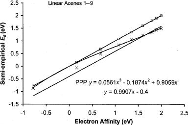
Figure 7.1 Plot of the semi-empirical Ea versus the experimental Ea for the linear acenes 1 to 9. The squares are the CURES-EC values that are equal to the experimental values within the uncertainties [8]. The x’s stand for the Pariser Parr Pople calculated values [10]. The latter have systematic uncertainties that vary with magnitude.

minimum value. The use of the AM1 procedure for the higher acenes will overestimate the Ea and the MINDO/3 procedure can underestimate the value. The pre-

dicted electron affinity for heptacene	is between 1.72 eV and 1.91 eV or
1.8 0.1 eV. The calculated value of	the ionization potential for heptacene is

6.14 eV, and when combined with the above Ea, it gives an electronegativity of 3.97 eV, consistent with earlier observations. The PPP value is 1.34 eV [10]. Likewise, the PPP values for octacene and novacene are lower than the CURES-EC values by 0.46 eV. The difference for benzene is 0.2 eV to 0.3 eV. As shown in Figure 7.1, this is an example in which the systematic uncertainty is not constant but depends on magnitude.

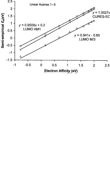
The calculated MINDO/3 LUMOs for these molecules are lower than the experimental Ea by 0.70 eV and for AM1 are higher than the experimental Ea by about 0.1 eV. These are shown in Figure 7.2. The systematic uncertainties remain constant. Figure 7.3 provides the optimum values of the VEa for the linear acenes. The VEa are between the AEa and MINDO/3 LUMO values. The calculated VEa for hexacene to novacene support the AEa values of 1.65 eV to 2.0 eV. The systematic difference is the rearrangement energy. It is approximately 0.2 eV for anthracene and above.

In both the AM1 and MINDO/3 procedures low-lying excited states are observed. Interestingly, in the case of naphthalene, the splitting is about 0.4 eV, and in the case of the AM1 procedure, one is negative by 0.2 eV, while the other is positive. More significant is the increase in the number of low-lying states that

SEMI-EMPIRICAL QUANTUM MECHANICAL CALCULATIONS

145

Figure 7.2 Plot of the semi-empirical Ea versus the experimental Ea for the linear acenes 1 to 9. The x’s are the CURES-EC values that are equal to the experimental values within the uncertainties. The circles are the calculated VEa and the triangles the LUMO. These are displaced from the CURES-EC values by a constant amount. This implies that the rearrangement energies are approximately the same for the linear acenes, as determined in [8] and this book.

Figure 7.3 Plot of the semi-empirical Ea versus the experimental Ea for the linear acenes 1 to 9. The x’s are the CURES-EC values that are equal to the experimental values within the uncertainties. The squares are the AM1 calculated with LUMO, while the triangles are the MINDO/3 LUMO. These are displaced from the CURES-EC values by a constant amount, as determined in [8] and this book.

146 CONSOLIDATING EXPERIMENTAL, THEORETICAL, AND EMPIRICAL DATA

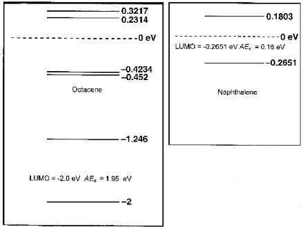
Figure 7.4 Lowest unoccupied molecular orbitals for naphthalene and octacene calculated using AM1. The values are negative, indicating a positive Ea. There are more positive Ea for octacene than naphthalene.

could accommodate the extra electron as the number of rings increased. These are illustrated in Figure 7.4 for naphthalene and octacene using AM1. For octacene there are four unoccupied orbitals with negative energies with a positive electron affinity by Koopman’s theorem. The energy of the LUMO is 2.0 eV and gives an Ea of 2.0 eV. The CURES-EC AEa is 1.90 eV. Several low-lying orbitals have small positive energies and could be involved in configuration interactions. These are related to the different types of C H bonds with different gas phase acidities. In the case of naphthalene these are the 1 and 2 C H bonds with gas phase acidities that differ by 3.1 kcal/mole or 0.14 eV [11–13].

The charge densities for the anions can be displayed in HYPERCHEM as illustrated in Figure 7.5, where the charges on C and H are shown for the naphthalene anion. The Values of the linear acenes vary from 0.06 to 0.26q for benzene to0.05 to 0.15q for naphthalene, to 0.04 to 0.18q for anthracene and tetracene. For pentacene the range is lowered to 0.03 to 0.14q. Thus, the solution energy differences should be smaller for the higher acenes and fullerenes. In predicting the reduction potential value for heptacene, this variation should be included. The reduction potential based on a value of 0.6 V versus Hg pool for hexacene is predicted to be 0.5 V versus the Hg pool. The value, if we assume a constant