Chen The electron capture detector

SEMI-EMPIRICAL QUANTUM MECHANICAL CALCULATIONS

147

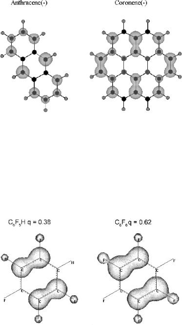
Figure 7.5 Charge densities on the anions of benzene and naphthalene calculated with MINDO/3. The localized charge is lower in naphthalene than benzene.

solution energy difference, is 0.4 V versus Hg pool. The reference energy of the Hg pool electrode is 4.15 V so that for heptacene with an Ea of 1.80 eV and a mdG

of 1.85 V, the E1=2 ¼ 4:15 þ 1:85 þ 1:80 ¼ 0:4 V.

The application of CURES-EC to CS2 illustrates a simple molecule where the geometry changes in the anion. The ECD data show two Ea at 0.85 eV and 0.6 eV. The neutral molecule is linear, while the anion is bent. The excited state Ea is the energy difference between the linear neutral and linear anion and is 0.6 eV. The MINDO/3(0000) energy difference between the linear neutral and bent anion is 0.81 eV. The optimum value is 0.88 eV for MINDO/3(2200). The photodetachment energy from the bent anion to the bent neutral is 1.2 eV, compared to the experimental 1.46 0.02 eV.

The linear acenes can also be used to illustrate the READS-TCT procedure. The first step in such a procedure is to establish the charge transfer for two identical molecules when one electron is added to the system. This is done for two anthracene molecules in Figure 7.6. The spin distributions are shown as a threedimensional plot along with the charge densities. The charge densities are the numbers in the background. The total charge on one of the species can be read from the HYPERCHEM window when one of the molecules is selected. When the species are the same, the charge and spin densities are equally distributed through space without a bridge or bond. For the heteromolecular systems a larger charge and spin distribution is on the molecule with the larger electron affinity. For the anthracene/naphthalene system this is 10 to 1. For higher consecutive acenes the ratio approaches 3 to 1 at heptacene and hexacene. For naphthalene to benzene it is 10 to 1, whereas for anthracene to benzene the charge on benzene is negligible. The READS (phenanthrene/naphthalene) is 3 to 1 for an electron affinity ratio of 0.30/0.17. For coronene/anthracene READS (C/A) is 2 to 1 as shown in Figure 7.7, where anthracene is selected and shows a total charge of 0.34. In Figure 7.8 the relative spin densities for these same two molecules can be seen. By calculating

148 CONSOLIDATING EXPERIMENTAL, THEORETICAL, AND EMPIRICAL DATA

Figure 7.6 Three-dimensional spin densities and charges for one electron distributed on two anthracene molecules calculated using MINDO/3. Both the spin densities and charge densities are equally distributed through space.

the READS (CS2/coronene) in the bent and linear forms of CS2, the Ea of coronene falls between the Ea of the bent and linear forms: READS (bent/C) ¼ (0.54/0.46), READS (linear/C) ¼ (0.2/0.8). The electron affinity of coronene is greater than 0.6 eV but less than 0.88 eV. This stands in contrast to the PES and collisional ionization values that are less than 0.6 eV [14–16].

Figure 7.7 Charges for one electron distributed on one anthracene and one coronene molecule calculated using MINDO/3. Seventy percent of the electron is localized on the coronene molecule, as indicated in the window when the anthracene molecule is selected.

SEMI-EMPIRICAL QUANTUM MECHANICAL CALCULATIONS

149

Figure 7.8 Three-dimensional spin densities and charges for one electron distributed on one anthracene and one coronene molecule calculated using MINDO/3.

A very important use of this technique is determining the relative electron affinities of multisubstituted compounds for which little data are available. For hexafluorobenzene and petafluorobenzene the READS (hexaF/pentaF) ¼ (0.611/0.389), while the value for READS (p-diF/FBz) ¼ (0.595/0.405) and READS(s-triF/ p-diF) ¼ (0.595/0.405). The sequential addition of a fluorine increases the Ea, and the READS values are relatively constant. The charge distributions are shown in Figure 7.9 for hexafluorobenzene and petafluorobenzene. The pentafluorobenzene value is 0.389q. The value for the hexafluorobenzene is the complement or 0.611q.

Figure 7.9 Charges for one electron distributed on hexafluorobenzene and pentafluorobenzene calculated using AM1. Sixty percent of the charge is localized on hexafluorobenzene by adding up the charges or selecting one molecule.

150 CONSOLIDATING EXPERIMENTAL, THEORETICAL, AND EMPIRICAL DATA

Figure 7.10 Three-dimensional spin densities for planar and distorted anions of cytosine calculated with AM1 [3].

The CURES-EC and READS-TCT procedures can be applied to more complicated biological molecules such as cytosine and thymine. The NH2 on cytosine is twisted out of the plane in the anion, as shown in Figure 7.10. The AM1(0000) Ea for the planar anion and neutral is 0.65 eV. The minimum AM1(0033) Ea is 0.3 eV. The energy of the planar form is 1,355.8 kcal/mole, whereas that in the global minimum is 1,360.73 kcal/mole. In order to go from the planar form that is a local minimum in the energy surface to the global minimum, the sample must be annealed. For the global minimum in the energy with the twisted NH2 group, the AM1(0033) Ea is 0.56 eV, which is equal to the values obtained in experiment. The two geometries can be seen in Figure 7.10, where the differences in the spin distributions may be easily visualized. In the global minimum there is spin density on the carbonyl group, whereas in the case of the planar anion none exists for the carbonyl group, but there is spin density on the C H group opposite the carbonyl group [17]. These changes are especially important for the GC hydrogen-bonded base pairs, as will be discussed in Chapter 12.

7.3MORSE POTENTIAL ENERGY CURVES

In 1963 negative-ion Morse parameters for the ground-state anions of Br2 and I2 were obtained by estimating D, re, and n from the VEa measured from charge transfer spectra and properties of the excited states of the neutral. Multiple excited states of I2( ) were characterized by D. R. Herschbach in 1966. He presented general forms for ionic Morse potential energy curves (HIMPEC). Nine total groups

MORSE POTENTIAL ENERGY CURVES

151

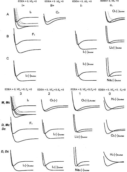
were based on dissociation or molecular ion formation in the Franck Condon region, the repulsive nature of the anion curves, the sign of the VEa, and the sign of EDEA ¼ D EaðXÞ. Herschbach described the HIMPEC as ‘‘a convenient qualitative classification of the types of XY( ) potential energy curves which may occur is given [see Figure 7.11 here]. . . . The category I or II is determined from the sign of the EDEA. In both cases A and B, the free anion is bound, but for B as well as the unbound case C, the vertical transition leads to dissociation’’ [2]. The ‘‘C’’ curves are slightly bound due to polarization forces. These are stronger than the attractions in He2, but weaker than the interactions responsible for dipole bound anions of molecules. However, there are several spaces where no curves can exist. Thus, the parameters for the classification were modified in 2001. For convenience the original classifications given in Chapter 2 are compared to the updated ones in Figure 7.11. The characterization of these Herschbach Morse groups is the first objective of this section.

The second objective will be to describe in detail the procedure for obtaining Morse potentials from diverse data using H2, I2, benzene, and naphthalene as examples. Hydrogen is chosen because it is the simplest homonuclear diatomic molecule and its adiabatic electron affinity corresponds to the polarization curve. Quantum mechanical calculations represent this as a free electron and molecule. Iodine is chosen because the electron impact distributions yield 12 curves. This splitting of the states is predicted theoretically for both I2( ) and Xe2(þ). The bond dissociation energies of the Xe2(þ) have been determined for these 10 states. Negativeion states not observed in the Xe2(þ) have been observed in I2( ) [18–25]. By using the split curves and absorption spectra of the negative ions, 10 excitedstate curves are defined. Benzene is chosen because the polarization anion is in the ground state like H2. Naphthalene is the first aromatic hydrocarbon with a positive valence-state electron affinity. Multiple low-lying negative-ion states of naphthalene have been observed, one of which has a negative electron affinity. Naphthalene has two distinct types of C H bonds for which two different gas phase acidities have been measured [11–13].

7.3.1Classification of Negative-Ion Morse Potentials

In the updated HIMPEC the sign of three independent metrics—the electron affinities Ea, the vertical electron affinities VEa, and the energy for dissociative electron attachment EDEA—gives 23 ¼ 8 possible curves. These are described in a symmetrical notation: MðmÞ and DðmÞ, m ¼ 0 to 3, where m is the number of positive metrics and M and D signify molecular anion formation and dissociation in a vertical transition. The EDEA is positive when the electron affinity is larger than the bond dissociation energy since it is EDEA ¼ EaðXÞ BDEXY . The Ea is the difference in energy between the individual anions and ground state of the neutral. By convention Ea are positive for exothermic reactions. The VEa are the energy differences for each anion in the geometry of the neutral. By definition the ground-state adiabatic Ea, AEa, is positive, but excited-state Ea and VEa can be negative or positive. By considering the rðe Þ-XY separation as a third dimension, eight subclasses

152 CONSOLIDATING EXPERIMENTAL, THEORETICAL, AND EMPIRICAL DATA

Figure 7.11 Original Hershbach ionic morse potential energy curves and the modified HIMPEC [2, 3]. The curves are calculated for the current best available data. The multiple curves for O2( ) and I2( ) are given to illustrate the relative positions of the curves. The specific example is the curve that is solid.

MORSE POTENTIAL ENERGY CURVES

153

can be defined as McðmÞ and DcðmÞ in which the ground state neutral crosses the anion curves to yield molecular ions or dissociation.

The electron affinities of many homonuclear diatomic molecules have been measured by anion photoelectron spectroscopy or photodetachment, but few Morse potential energy curves have been calculated. The AEa for H2 and N2 are positive but small since the ground-state anions correspond to long-range ion polarization states. The anions are as follows: H2 [M(0), Mc(0); D, Dc(0)]; Li2 [M(2), Mc(2), D(1)]; C2 [M(2), Mc(2)]; O2 [M(2, 1), Mc(2, 1, 0); D(0), Dc(0)]; F2 [D(3, 2), Dc(3, 2)]; Na2 [M(2), Mc(2); D(1), Dc(1)]; and I2 [M(3), Mc(3); D(3, 2), Dc(3, 2)] illustrate the classes as shown in Figure 7.11.

The Morse potentials for the neutral and HIMPEC as referenced to zero energy at infinite separation are given by

UðX2Þ ¼ 2DeðX2Þ expð bðr reÞÞ þ 2DeðX2Þ expð 2bðr reÞÞ	ð7:1Þ
UðX2 Þ ¼ 2kADeðX2Þ expð kBbðr reÞÞ þ kRDeðX2Þ expð 2kBbðr reÞÞ
EaðXÞ þ EðX Þ	ð7:2Þ

where DeðX2Þ is the spectroscopic dissociation energy; r is the internuclear separation; re ¼ r at the minimum of UðX2Þ; EaðXÞ is the electron affinity of X; EðX Þ is the excitation energy; bðX2Þ ¼ neð2p2mðX2Þ=DeðX2ÞÞ1=2; m is the reduced mass; kA, and kB, and kR are dimensionless constants. The variation in the reduced mass of the anion occurs in the kB term since kB ¼ bðX2ð ÞÞ=bðX2Þ. The HIMPEC are also Morse potentials, and the negative-ion parameters can be calculated from those of the neutral and dimensionless constants using these equations:

DeðX2ð ÞÞ ¼ ½kA2 =kR&DeðX2Þ	ð7:3Þ
reðX2ð ÞÞ ¼ ½lnðkR=kAÞ&=½kBbðX2Þ& þ reðX2Þ	ð7:4Þ
neðX2ð ÞÞ ¼ ½kAkB=kR1=2&neðX2Þ	ð7:5Þ
VEa ¼ DeðX2Þð1 2kA þ kRÞ EAðXÞ þ EðX Þ 1=2hneðx2Þ	ð7:6Þ

The negative-ion properties have not been measured directly. Therefore, it is necessary to combine data from different sources to obtain the dimensionless parameters to define the curves. Three data points on the curve will define a negative-ion curve. The Herschbach metrics EDEA, Ea, and VEa give kA and kR from equations 7.3 and 7.6 since the DeðX2ð ÞÞ are directly related to the Ea and EDEA. This only gives two constants since the EDEA is a displacement of the negative-ion curve from the neutral, and a third point is required. The neðX2ð ÞÞ or reðX2ð ÞÞ gives kB from equation 7.4 or 7.5 to define the anion Morse potentials.

7.3.2The Negative-Ion States of H2

The first step in assigning the experimental Ea to electronic states is to determine the number of theoretical states. The H2 anion has a polarization ground state and

154 CONSOLIDATING EXPERIMENTAL, THEORETICAL, AND EMPIRICAL DATA

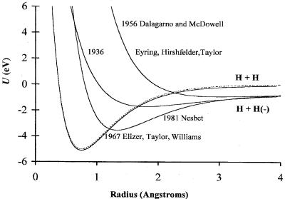
Figure 7.12 Historical Morse potential energy curves for H2 and its anions, dating back to 1936 [25], 1956 for the excited state [26], 1967 for the polarization ground state [27], and 1981 for the valence excited state [28].

two covalent states. The ground state is a ‘‘neutral molecule plus free electron.’’ Because of the simplicity of the H2( ) ions, many attempts have been made to characterize them. Morse parameters D, r, and n) (0.9 eV, 190 nm, 1,127 cm 1 and 0.16 eV, 300 nm, 600 cm 1) were calculated for the bonding and antibonding states in 1936 and 1956. In 1967 a curve for the polarization state was calculated, but the bond dissociation energy was less than that of the neutral, giving it a negative Ea. In 1967 and 1981 improved bonding curves were calculated; however, the dissociation energy remained too small. One net bonding electron is present in H2( ), as in He2(þ) and H2(þ). The neutral has two bonding electrons, and the dissociation energy of the anion is one-half that of the neutral or De ¼ 2:65 eV. The bond dissociation energy of the polarization state should be slightly larger than that for the neutral and the internuclear distance and frequencies should be about the same. When we use these bond dissociation energies and the calculated frequencies and internuclear distances, the Morse potentials for the anion states of H2( ) can be calculated. These are illustrated in Figure 7.12, along with the 1936 curve formulated by Eyring Hirschfelder and Taylor. They can be compared with the current ‘‘best’’ curves shown in Figure 7.13 [26–29].

Until recently, the only experimental data that were available for H2( ) were electron impact distributions for the formation of H( ). The H( ) peaks were observed with an abrupt onset at EDEA ¼ 3.75 eV, an onset at 7 eV, and a peak at 10 eV [30]. These data are shown in Figure 7.14 with the calculated distributions.

MORSE POTENTIAL ENERGY CURVES

155

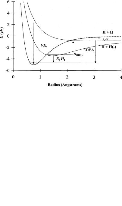
Figure 7.13 Current ‘‘best’’ Morse potential energy curves for H2 and its anions, from [30–32].

Electron scattering data give a VEa of 3.3 eV for the bonding state [31]. The ESR spectrum of the valence-state anion has been observed in irradiated solid H2 [32]. The combination of these data yields re ¼ 153 pm and ne 1,700 cm 1 for the bonding valence-state anion. The H( ) distribution and an assumed dissociation energy

Figure 7.14 Electron impact spectrum calculated from the current ‘‘best’’ Morse potential energy curves for H2 and H2( ) shown in Figure 7.13, from [30].

156 CONSOLIDATING EXPERIMENTAL, THEORETICAL, AND EMPIRICAL DATA

TABLE 7.3 Morse Parameters, Dimensionless Constants, and Experimental Data for Neutral and Ionic H2 and He2(þ)

					kA	kB	kR	D0 (eV)	re (pm)	ne (cm 1)
		þ		u
He2(			)	2 þ	1.11	0.62	2.40	2.58	108	1,964
	þ			2 gþ	0.16	0.49	1.38	0.08	190	300
				u
H2(			)	2 þ	0.84	0.69	1.26	2.79	106	2,250
H2 Neutral					1.00	1.00	1.00	5.01	75.4	4,395
H2( )				Polar	1.00	1.00	1.00	5.1	75.4	4,395
				2 uþ	1.07	0.53	2.14	2.58	145	700
				2 gþ	0.12	0.56	0.99	0.05	280	285

of 0.05 eV were used to calculate the antibonding Morse potential [31]. The bonding curve is an M(0) curve, while the antibonding curve is a D(0) curve. The Morse parameters and dimensionless constants for the neutral and anions of H2 and the cations of H2 and He2 are in presented Table 7.3. The attractive term kA ¼ 1, is about the same in the bonding valence-state anion, but the repulsive term kR is doubled. In the antibonding state the attractive term is diminished, while that for the repulsive term is the same as for the neutral. The radius of H( ) is obtained from reðH2ð Þ rðHÞ ¼ 145 38 ¼ 107 pm.

7.3.3The Negative-Ion States of I2

Twelve negative-ion states for I2 have been predicted [25]. The ground-state curves have been completely characterized by photon experiments. This is the only X2ð Þ ground-state curve so well characterized [23]. The bond dissociation energy is the same for the ground state of iso-electronic Xe2ðþÞ [3, 18, 21]. Electron impact data define the vertical electron affinities of 10 states, while the bond dissociation energies of the excited states of isoelectronic Xe2(þ) define excited-state Ea. One excited-state curve with a much lower bond dissociation energy than measured for Xe2(þ) has been observed in photon experiments [24]. The third point on some curves is the peak in the absorption spectra of the ground-state anion. The Ea of one state can be calculated from the observed bond dissociation energy. For all the VEa the I( ) distributions have been measured [19]. This defines the slope of the excited-state curves in the Franck Condon region. Finally, the activation energies of the thermal electron attachment to two excited states have been measured in ECD experiments [8, 22]. Thus, some of these curves are overdetermined with five data points. The values of kA, kB, and kR could be calculated using the analytical expressions 7.3 to 7.6. However, this is not done. Instead, the electron impact curves are fit to the Ea and VEa to give the ion distribution. Then the calculated absorption peak is adjusted to determine the experimental values. An isobestic point is assumed for several curves since not all the absorption peaks have