Baer M., Billing G.D. (eds.) - The role of degenerate states in chemistry (Adv.Chem.Phys. special issue, Wiley, 2002)

18	m. s. child

subsequent discussions. In its linear variant, with l ¼ 0 in the above equations, it provided the first example of geometric phase, plus a less familiar half-integral quantum number [2]. The effects of spin–orbit coupling on geometric phase [21,24] are also conveniently illustrated. Addition of the quadratic terms in Eq. (7) or (8) is of interest in introducing a threefold corrugation on the lower adiabatic potential surface leading to an ‘‘inverted’’ pattern of vibronic multiplets (E levels below A, in the lowest triplet), which is one of the clearest experimental manifestations of geometric phase [11]. There is also an interesting question concerning the relative magnitudes of the linear and quadratic terms in Eqs. (7) and (8). We shall find that there is no geometric phase effect unless k ¼6 0, which raises questions as to the nature of its disappearance as k=l ! 0:

A.The Linear Jahn–Teller Effect

It is convenient to discuss the linear Jahn–Teller model in the scaled complex representation

h

kre if

ð61Þ

H ¼ kre0if

h0

where

1

q

r

q

1

q2

1

r2

h0 ¼

þ

ð62Þ

2r

qr

qr

2r2

qf2

2

rather than in the real representation in Eq. (20). It is readily verified, by ignoring the kinetic energy terms, that the eigensurfaces take the form

W ¼	1		r2 kr					ð63Þ
		2
with single-valued eigenstates
	1				1			ð64Þ
jn i ¼ p2						eif

Substitution in Eq. (33) therefore yields gC ¼ p, in agreement with the result obtained from the real representation of the Hamiltonian in Eq. (20).

Figure 1a shows that the eigensurfaces form an interconnected double sheet,

the	lower member of which has a ring of equivalent minima at r					¼	k	and
		1	2	:	As expected angular momentum is conserved, but			the
W ¼		2 k				with
complication					that it is vibronic, rather than purely vibrational in character,

early perspectives on geometric phase

19

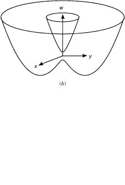
Figure 1. Adiabatic potential surfaces (a) for the linear E E case and (b) for a 2E state with linear Jahn–Teller coupling and spin–orbit coupling to a 2A state.

because it may be confirmed that the operator
^	^	q
^| ¼ lz þ sz	lz ¼ i	qf	ð65Þ

commutes with H; and ^| includes an electronic component, sz, as well as the

^ ^

vibrational term lz: The single valued eigenstates of | , belonging to the upper and lower potential surfaces, may be obtained by multiplying Eq. (64) by eið j 1=2Þf; thus

1		ei j 1=2Þf			j ¼	1		3		5			ð66Þ
juj ðfÞi ¼ p2			eðið jþ1=2Þf			2		; 2		; 2 . . .

They must be coupled by separate radial factors in a full calculation [2] but, to the extent that non-adiabatic coupling between the upper and lower

20	m. s. child

surfaces is neglected, the total lower adiabatic wave function may be expressed as

j i ¼ r 1=2juj ðfÞijv ðrÞi

ð67Þ

with the radial wave function on the lower adiabatic surface, jv ðrÞi, taken as an eigenstate of the radial operator

^

1 q2

j2

1

2

hr ¼

þ

þ

r

kr

ð68Þ

2r

qr2

2r2

2

For large k, the approximate potential minimum lies at r ¼ k and the lower vibronic eigenvalues are given by [2]

	k2		v þ	1	þ	j2
Ev j ¼		þ					ð69Þ
	2			2		2k2

The presence of the half-odd quantum number j in Eq. (69) is potentially a physically measurable consequence of geometric phase, which was first claimed to have been detected in the spectrum of Na3 [16]. The situation is, however, quite complicated and the first unambiguous evidence for geometric phase in Na3 was reported only in 1999 [17].

B.Spin–Orbit Coupling in a 2E State

The effects of spin–orbit coupling on geometric phase may be illustrated by imagining the vibronic coupling between the two Kramers doublets arising from a 2E state, spin–orbit coupled to one of symmetry 2A: The formulation given below follows Stone [24]. The four 2E components are denoted by jeþai, je ai, jeþbi, je bi, and those of 2A by je0ai, je0bi: The spin–orbit coupling operator has nonzero matrix elements

heþbjHsoje0ai ¼ he ajHsoje0bi

ð70Þ

giving rise to a second-order splitting, of say 2 , between one Kramers doublet, jeþai, je bi, and the other, je ai, jeþbi: There is also a spin-preserving vibronic coupling term, of the form in Eq. (61), giving rise to a Hamiltonian of the form

H	¼		h0 þ	kre if		ð	71	Þ
			kreif	h0

for one coupled pair and the complex conjugate form for the other. Notice

that Eq. (71) conforms to Eq. (13) with w	¼	, u	¼	kre if, and v	¼	0. The

early perspectives on geometric phase

21

eigensurfaces now take the forms

¼	1	r2	p	ð Þ
W	2		k2r2 þ 2	72

with an avoided conical intersection, as shown in Figure 1b.

It is convenient, for comparison with Section V.A, to employ substitutions

¼ rðrÞcos yðrÞ	kr ¼ rðrÞsin yðrÞ	tan yðrÞ ¼	kr	ð73Þ

which convert the Hamiltonian in Eq. (71) to the form in Eq. (44). Comparison with Eq. (50) shows that the geometric phase, for a cycle of constant radius, r, is given by

gC ¼ ð1 cos yðrÞÞp	ð74Þ
It reverts to the unspin–orbit modified value, gC ¼ p, for paths such	that
kr , but vanishes as r ! 0:	^

Reverting to the vibronic structure, the operator ^| again commutes with H, and the analogue of the lower adiabatic eigenstate of ^| in Eq. (66) becomes

1		sin y eið j 1=2Þf	!	1			3		5
		2										ð75Þ
		2
juj ðr; fÞi ¼ p2	cos y eið jþ1=2Þf			j ¼ 2		;	2		; 2 . . .

where the r dependence of juj ðr; fÞi comes from that of yðrÞ: There is also an equivalent complex conjugate eigenstate of the complex conjugate Hamiltonian to that in Eq. (71). One finds after some manipulation that

huj ðr; fÞjh0jr 1=2uj ðr; fÞi

2

1

2

j2

j cos

1

dy

¼ r 1=2(

q

þ

þ

y

þ W ðrÞ þ

)

ð76Þ

2

qr2

2r2

8

dr

The radial factor in the total wave function

j i ¼ r 1=2juj ðfÞijv ðrÞi

ð77Þ

must therefore be an eigenstate of

1 q2

j2

j cos y

1

dy

2

h^r ¼

þ

þ

þ W ðrÞ þ

ð78Þ

2

qr2

2r2

8

dr

22	m. s. child

The principal differences from Eq. (68) lie in the form of the potential W ðrÞ and in the presence of the term j cos y, of which the latter arises from the dependence

^

of the geometric phase on the radius of the encircling path. The eigenvalues of hr are no longer doubly degenerate, but a precisely equivalent Kramer’s twin radial Hamiltonian may be derived from the complex conjugate of Eq. (71).

C.The Quadratic Jahn–Teller Effect

The quadratic Jahn–Teller effect is switched on by including the quadratic terms in Eq. (7); thus, with the inclusion of the additional diagonal Hamiltonian h0,

H	¼	h0	kre if þ lr2e2if		ð	79	Þ
		kreif þ lr2e 2if	h0

The eigensurfaces are given by

ð	Þ ¼	1	r2		p	ð Þ
W r; f		2			r k2 þ 2klr cos 3f þ l2r2	80

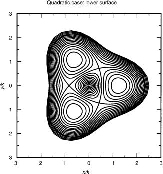
with a threefold corrugation around the minimum of W ðrÞ, in place of the line of continuous minima in Figure 1. The three absolute minima in Figure 2, at f ¼ 0; 2p=3, correspond to three equivalent isosceles distortions of an initially equilateral triangular molecule.

There is no simple general form for the adiabatic eigenvectors, except in the limits, k ¼ 0 and l ¼ 0, when, for example,

jx i ¼	e if=2	!	l ¼ 0
	eif=2

!

e if

¼ k ¼ 0 ð81Þeif

In the first case, jx i changes sign as f increases to j þ 2p, while in the second, jx i is single valued. There is therefore a geometric phase of p, for lr k, but no geometric phase in the opposite limit, lr k: The interesting questions concern (1) the effects of the corrugations on the vibronic eigenvalues; and (2) the origin of the change in geometric phase behavior as the ratio lr=k increases.

The first of these questions is deferred to Section VI. The second is addressed by considering the degeneracy condition Wþðr; fÞ ¼ W ðr; fÞ: One solution lies at r ¼ 0, and there are three others at r ¼ k=l and f ¼ p; p=3 [30,31]. A circuit of f with r < k=l therefore encloses a single degenerate point, which accounts for the ‘‘normal’’ sign change, e ip ¼ 1, whereas as circuit with r > k=l encloses four degenerate points, with no sign change because e 4ip ¼ 1:

early perspectives on geometric phase

23

Figure 2. Contours of the lower potential surface in the quadratic E E Jahn–Teller case.

Any proper treatment of the dynamics, including motion in the r variable therefore requires knowledge of the position of the minima of W ðr; fÞ, which are found to lie at r ¼ k=ð1 2l2Þ [units are dictated by the form of the scaled

restoring term r2=2 in Eq. (80)]. The potential minima therefore lie inside the p

critical circle r ¼ k=l if l < 1= 3 and outside it if the sense of the inequality is dynamics, in the sense to be discussed below, may

reversed. Single surface
therefore be assumed to apply with a geometric phase of p if l 1=p3, and
with no geometric phase if l 1=p3: Cases with l A1=p3, with significant
wave function amplitude at the degenerate				points with	r	k		l, cannot be
					¼		=
validly treated in an adiabatic approximation.
VI. SINGLE-SURFACE NUCLEAR DYNAMICS
Given the full-Hamiltonian
	^2
Hðq; QÞ ¼ X		P
		i	rQ2 i	þ Helðq; QÞ				ð82Þ
		2mi

24				m. s. child
and adiabatic eigenstates jnðq; QÞi, such that
				Helðq; QÞjnðq; QÞi ¼ WðQÞjnðq; QÞi	ð83Þ
the Born–Oppenheimer approximation to the total wave function,
				j ðq; QÞi ¼ jnðq; QÞijvðQÞi	ð84Þ
requires that
1			2	2
X			½P^i	þ 2hnjP^ijni P^i þ hnjP^i jni& þ WðQÞ jvðQÞi ¼ EjvðQÞi ð85Þ
	2mi

with appropriate boundary conditions on the vibrational factors jvðQÞi. As discussed in Section III, coupling terms of the form

n	m	hnjrQHeljmi	ð	86	Þ
h	jrQj i ¼	WnðQÞ WmðQÞ

have been neglected in the derivation of Eq. (85). The assumption is that the wave function has negligible amplitude in the vicinity of any points at which WðQÞ has a close degeneracy with any other eigensurface.

Geometric phase complications necessarily arise, however, whenever the nuclear wave function has significant amplitude on a loop around an isolated degeneracy. They can be treated in two ways, according to whether the adiabatic eigenstate jnðq; QÞi is taken to be multivalued or single-valued around the loop in nuclear coordinate space Q: Illustrations are given below for the two different approaches. The first concerns the energy ordering of the vibronic eigenstates arising from a strong quadratic Jahn–Teller effect [11]. The second outlines the vector potential approach, due to Mead and Truhlar [10], with applications to the above E E linear Jahn–Teller problems and to scattering problems involving identical nuclei.

A.The Ordering of Vibronic Multiplets

It was seen in Section V.C that quadratic Jahn–Teller coupling terms result in a threefold corrugation around the minimum energy path on the lower potential surface W ðQÞ and that there is a geometric phase, gC ¼ p, provided that the radius of the minimum energy path satisfies r < k=l: We now consider the influence of geometric phase on the relative energies of the (A; E) symmetry levels in different tunneling triplets. The solution, due to Ham [11], applies band theory arguments to assess the influence of antiperiodic, cðf þ 2pÞ ¼ cðfÞ,

early perspectives on geometric phase

25

boundary conditions on solutions of the threefold periodic angular equation

	h2 d2					2
				þ E VðfÞ cðfÞ ¼ 0	V f þ		p	¼ VðfÞ ð87Þ
	2m		df2				3

Note that there is no first derivative term in Eq. (87), because the first line of Eq. (81) ensures that hxjq=qfjxi ¼ 0:

The first strand of Ham’s argument [11] is that VðfÞ supports continuous bands of Floquet states, with wave functions of the form

ckðfÞ ¼ eikðEÞfxðfÞ

ð88Þ

where xðfÞ has the same periodicity as VðfÞ [32]. Elements of Floquet theory, collected in the appendix, show that the spectrum is bounded by 32 < k 0 32 , and that the dispersion curves, EðkÞ obtained by inversion of kðEÞ in Eq. (88), have turning points at k ¼ 0 and k ¼ 32.

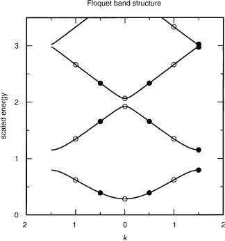
A second constraint is that the relative order of the critical energies at k ¼ 0 and k ¼ 32 is invariant to the presence or absence of the potential VðfÞ [11]: Equation (A.6) shows that the free motion band structure can be folded onto the interval 32 < k 0 32. Consequently, preservation of relative energy orderings at k ¼ 0 and k ¼ 32 implies a band structure for VðfÞ ¼6 0, with the form shown in Figure 3.

The question of vibronic energy ordering, with and without geometric phase, now turns on the appropriate values of k in Eq. (88), bearing in mind that all energy levels are doubly degenerate except those at k ¼ 0 and k ¼ 32. Normal periodic boundary conditions require integral k, with Eð0Þ < Eð 1Þ, in the lowest energy band. However, introduction of a sign change in ckðfÞ, to compensate the electronic geometric phase factor, introduces half odd-integral values of k, with Eð 12Þ < Eð32Þ. This ordering is seen from Figure 3 to be reversed and restored in the successively excited bands. It may also be noted that an explicit calculation of the lowest 89 vibrational levels of Na3 [33] confirms that the ordering of vibronic energy levels is the clearest observable molecular manifestation of geometric phase.

B.Vector-Potential Theory: The Molecular Aharonov–Bohm Effect

Mead and Truhlar [10] broke new ground by showing how geometric phase effects can be systematically accommodated in scattering as well as bound state problems. The assumptions are that the adiabatic Hamiltonian is real and that there is a single isolated degeneracy; hence the eigenstates jnðq; QÞi of Eq. (83) may be taken in the form

jnðq; QÞi ¼ eicðQÞjxðq; QÞi

ð89Þ

26	m. s. child

Figure 3. Floquet band structure for a threefold cyclic barrier (a) in the plane wave case after using Eq. (A.11) to fold the band onto the interval 32 < k 0 32; and (b) in the presence of a threefold potential barrier. Open circles in case (b) mark the eigenvalues at k ¼ 0; 1, consistent with periodic boundary conditions. Closed circles mark those at k ¼ 12 ; 32, consistent with sign-changing boundary conditions. The point k ¼ 32 is assumed to be excluded from the band.

where jxðq; QÞi is real, and cðQÞ is designed to ensure that jnðq; QÞi valued around the degeneracy. Consequently, Eq. (85) takes the form

X	1	½fP^i aig2	2	jxi& þ WðQÞ jvðQÞi ¼ EjvðQÞi
			þ hxjP^i
	2mi

where

is single

ð90Þ

ai ¼ hrQi c

ð91Þ

The term ai therefore plays the role of a vector potential in electromagnetic theory, with a particularly close connection with the Aharonov–Bohm effect, associated with adiabatic motion of a charged quantal system around a magnetic

early perspectives on geometric phase

27

flux line [12], a connection that has led to the phrase molecular Aharonov–Bohm effect [34,35] for the influence of ai on the nuclear dynamics. Note also that single valuedness of jnðq; QÞi allows considerable ambiguity in the definition of

cðQÞ, but it is easily verified that the					substitution of ~		Q for	Q merely alters
					~	cð	Þ	cð Þ
the phase of	j	ð	Þi	by a factor eiðc cÞ, without altering the essential dynamics:
		v Q

The simplest choice cðQÞ ¼ mf, where m is a half-odd integer and f is an angle measured around the degeneracy, is therefore normally employed in molecular Aharonov–Bohm theory.

An advantage of Eq. (90) for computational purposes is that the solutions are subject to single-valued boundary conditions. It is also readily verified that inclusion of an additional factor ei cðQÞ on the right-hand side of Eq. (89) adds a

term ai ¼ hrQi	c to the vector potential, which leads in turn to a comp-
ensating factor e i	cðQÞ in the nuclear wave function. The total wave function is
therefore invariant to changes in such phase factors.

We now consider the connection between the preceding equations and the theory of Aharonov et al. [18] [see Eqs. (51)–(60)]. The tempting similarity between the structures of Eqs. (56) and (90), hides a fundamental difference in the roles of the vector operator A in Eq. (56) and the vector potential a in Eq. (90). The former is defined, in the adiabatic partitioning scheme, as a strictly off-diagonal operator, with elements hmjAjni ¼ hmjPjni, thereby ensuring that ðP AÞ is diagonal. By contrast, the Mead–Truhlar vector potential a arises from the influence of nonzero diagonal elements, hnjPjni on the nuclear equation for jvi, an aspect of the problem not addressed by Arahonov et al. [18]. Suppose, however, that Eq. (56) was contracted between hnj and jnijvi in order to handle the adiabatic nuclear dynamics within the Aharonov scheme. The

result becomes
1		hnjP2jnijvi ¼	1	hhnjðP AÞ2jnijvi þ hnjA2jnijvii	ð92Þ
	2m		2m

Given a real electronic Hamiltonian, with single-valued adiabatic eigenstates of the form jni ¼ eicðQÞjxni and jxmi, the matrix elements of A become

hmjAjni ¼ hxmjAjxni ¼ hxmjPjxni

ð93Þ

so that

XX

hnjA2jni ¼	hnjAjmihmjAjni ¼ hxnjPjxmihxmjPjxni ¼ hxnjP2jxni ð94Þ
m	m

The sum over all m is justified by the fact that the diagonal elements hxnjPjxni vanish in a real representation. It is also evident from the factorization of jni and