Friesner R.A. (ed.) - Advances in chemical physics, computational methods for protein folding (2002)(en)

396	john l. klepeis et al.

determined and then sorted. Connections between this point and all points which are within the cutoff distance are noted, so that equivalence classes may be determined. Then the pairs consisting of this point and each of the next N points (N is the coordination number), along with their mutual distances, are added to a ‘‘pairs’’ list. After all points have been considered and the equivalence classes are determined (class-wise), duplicate pairs are discarded from the ‘‘pairs’’ list, and then the points are generated as described above.

The most CPU-intensive part of the algorithm is the generation of a list of distances between a given point and every other point, along with the sorting of that list. In the parallel version of this algorithm, the master process sends the set of points to each slave process so that they will know what to do. While the master process is carrying out the remainder of the algorithm, each slave process calculates the distances between a given point and every other point and then sorts the list. As each point is considered in turn, the master process cycles through the slave processes, receiving the needed distances from each one.

Clustering. The number of minima and transition states can be reduced by ‘‘clustering’’ them—that is, by identifying points that lie within a specified distance of one another with a single point. The first point in the set of points to be clustered is selected as a cluster center and compared with every other point. Points within a certain cutoff distance from the selected cluster center are identified as belonging to that cluster and taken out of circulation. The next point in the set that is not yet part of any cluster is selected as the next cluster center, and it is compared with all other points not yet part of any cluster. The algorithm continues this way until all points have been assigned to a cluster.

Note that the clusters generated by this algorithm have the property that the cluster centers used to generate them appear earlier than all of the other points in the cluster. Thus, by first sorting the set in increasing order of potential energy, we can guarantee that each cluster will be represented by its lowestenergy member and, in particular, that the global minimum energy point will be among the cluster centers.

Minima should be clustered first using the algorithm as described above. The connectivities between the transition states and the minima they connect should then be redefined so that transition states connect the cluster centers associated with the minima they actually connect. Then the transition states can be clustered using the algorithm as described above with one additional caveat: One transition state cannot be identified as belonging to a cluster centered by another transition state unless they connect the same two minima (clusters).

The most CPU intensive part of the algorithm is the calculation of distances between selected cluster centers and all other nonclustered points. The parallel version of this algorithm runs as follows. The points are first sorted, and then they are shipped from the master process to each slave process. The master

deterministic global optimization and ab initio approaches 397

process sends the first cluster center to one of the slave processes which begins comparing that point to all of the remaining points in the set. As cluster matches occur, results are reported back to the master process that records the clustering information. The master process continues sending cluster centers to available slave processes and awaits reports of clustering until all points have been clustered.

The situation is complicated by the fact that the master process cannot send a new cluster center to another slave process until it is established that the potential cluster center does not belong to a cluster defined by a previous cluster center. As long as each slave process performs the comparisons in order, the master process will be able to deduce that the next unclustered point should be regarded as a new cluster center as soon as all active slave processes have reported progress beyond that point. To facilitate this process, each slave process reports its progress back to the master process at well-defined intervals,5 in addition to those instances where a cluster match is found.

3.Methods for Analyzing the Potential Energy Surface

Vibrational Frequencies Calculation. The vibrational frequencies are determined by solving the generalized eigenvalue problem

ðH ð2pnÞ2IÞx ¼ 0

where H is the Hessian and I is the generalized inertia tensor, defined so that the kinetic energy of the system is given by

K	¼	1	X	dxi	Iij	dxj
		2 i; j dt				dt

The inertia tensor is calculated by first calculating drj=dxi for j ¼ 1; . . . ; 3Na and i ¼ 1; . . . ; Nx by finite differencing and then using the following formula:

			3Na	drj drj
	Iii0	¼	X mj
				dxi dxi0
			j¼1

where mj is the mass of the j=3-th atom.

This makes use of the Cartesian coordinate functions rðxÞ. The formulae above depend on the Cartesian coordinates being physically correct.

5A geometric sequence is used so as to generate a number of early reports without generated an enormous number of total reports. Thus, reports are sent back after comparing the cluster center to the next 1, 5, 52, 53, . . . points.

Y 2 sinh hni

398	john l. klepeis et al.

Unfortunately, most methods of generating Cartesian coordinates from generalized coordinates (in our case, dihedral angles) involve fixing the positions and orientations of specific atoms, which leads to the introduction of unphysical forces and torques being applied to the molecule. We eliminate these unphysical forces by augmenting the set of generalized coordinates to include overall translation and rotation coordinates, calculating the vibrational frequencies using the above methods, and then discarding the six zero-mode frequencies (which must exist). The resulting vibrational frequencies are physically correct.

Vibrational frequencies can be computed at the end of an eigenmodefollowing search at little cost, because the Hessian has already been generated. Alternatively, the vibrational frequencies can be calculated all at once after the minima and saddles have all been found. In the latter case, the calculation can be run in parallel by distributing the work to each process, having them calculate the frequencies, and then having them pass the results back to the master process.

Free Energy Calculation. The free energy for a given stationary point is defined as follows:

F ¼ E TSvib

The vibrational entropy is calculated from the vibrational frequencies by employing the Classical Harmonic Oscillator approximation

Svib ¼ k ln

Yhni

i kT

where the product is taken over all vibrational frequencies. For saddle points of order 1 or higher, the negative eigenvalue modes are not counted as ‘‘vibrational modes.’’

Other methods of calculating the vibrational entropy exist, but are not currently implemented. Perhaps the simplest is the Quantum Harmonic Oscillator approximation:

Svib ¼ k ln

2kT

i

Anharmonic methods exist in the literature [163,164].

Equilibrium Probabilities. Equilibrium probabilities are calculated from the contribution to the partition function from each minimum, which can be expressed in terms of its free energy:

e Fi=kT Pi ¼ Pj e Fj=kT

deterministic global optimization and ab initio approaches 399

The minimum free energy over the entire system is first subtracted off in order to prevent overflow/underflow problems that could arise from modest nonzero free energies (positive or negative).

Average values (as well as standard deviations) of any quantity can now be computed at equilibrium:

X hqi ¼ qiPi

i

sq ¼ ðhq2i hqi2Þ1=2

Temperature derivatives are also possible:

dhqi ¼ hqEi hqihEi dT kT2

assuming that qi does not depend explicitly on temperature. In particular, the specific heat Cv ¼ dhEi=dT can be calculated.

Transition Rates. Transition rates are computed by Rice–Ramsperger–Kassel– Marcus (RRKM) theory. Each transition state is associated with two rates:

Wi!ts!j ¼ kTh e ðFts FiÞ=kT

Wj!ts!i ¼ kTh e ðFts FjÞ=kT

These rates are collected together in a (sparse) matrix:

X

Wij ¼ Wj!ts!i ts

Time-Dependent Probabilities (Master Equation). The time development of occupation probabilities can be determined by solving the Master equation:

	dPi	XWijPj		ð	XWji	Pi	X wijPj
	dt
		¼	j		Þ		¼
					j		j
where
		wij	Wij			ðif i ¼6 jÞ
			¼ Pi0 Wi0i			ðif i ¼ jÞ

400	john l. klepeis et al.

Solving the Master equation involves determining the eigenvalues and eigenvectors of the (nonsymmetric, but easily symmetrizable) matrix w:

X

wijuðjkÞ ¼ lðkÞuðikÞ

j

The occupation probabilities as a function of time can be computed (and, e.g., plotted):

PjðtÞ ¼ X akelðkÞtuðjkÞ

k

where the coefficients ak are determined from the initial conditions Pjð0Þ. The time constants are determined from the eigenvalues

tk ¼ 1=lðkÞ

One of the eigenvalues is zero, which corresponds to the equilibrium probability distribution (t ¼ 1). The remaining eigenvalues will be negative.

Average values (as well as standard deviations) of any quantity can now be computed as a function of time (and, e.g., plotted):

hqiðtÞ ¼ X qjPjðtÞ ¼ X akðXqjuðjkÞÞelðkÞt

j k j

sqðtÞ ¼ ðhq2iðtÞ hqiðtÞ2Þ1=2

Solving the Master equation requires the diagonalization of a matrix whose size is the number of minima in the system. This is an extraordinarily expensive operation and may be prohibitive in both space and time resources required. A 4000 4000 matrix requires 128 megabytes of storage and generally requires about a day of CPU time to diagonalize. There is no parallel algorithm available for this operation.

Pathways. Each transition state connects two minima on the potential energy surface. A pathway between two minima is defined as a series of such connections:

initial state ! ts ! min ! ts ! ! ts ! min ! ts ! final state

The set of all (nonlooping) pathways from one minimum to another can be found by an exhaustive search. We begin at the initial state and move to each minimum that is connected to the initial state. For each such minimum, we recursively

deterministic global optimization and ab initio approaches 401

explore all minima connected to that minimum, taking care not to visit a given minimum more than once along the same pathway. When the final state is reached, the pathway is reported. When all possible routes have been explored, the algorithm terminates.

For any reasonably sized system of minima and transition states, the number of possible nonlooping pathways between any two minima is likely to be prohibitively large. There are several criteria that can be applied to reduce the number of pathways:

1.Monotonicity in any specified quantity (such as energy or free energy). Transitions are ignored if they violate the proposed monotonicity.

2.Maximum length (i.e., maximum number of minima, including the initial and final state, visited along the pathway).

3.Minimum transition rate. Transitions are ignored if they are slower than this cutoff rate.

The following information is available during a pathway calculation:

1.The set of minima and/or transition states visited along the way by at least one of the pathways.

2.Transition rates for each transition taken along a given pathway.

3.An overall ‘‘transition time’’ for a given pathway. This is determined by

(a)solving the Master equation over the minima and transition states involved in that one pathway alone and (b) using the lifetime of the longest-lived transient probability eigenvector.

4.Values of any number of quantities for each minimum visited along a given pathway.

5.The two reaction coordinate indicator values associated with any number of quantities along each given pathway (explained below).

6.The average value and standard deviation of any number of quantities over all pathways, at a fixed position along the pathways.

7.The average value and standard deviation of the two reaction coordinate indicators over all the pathways (explained below).

For a given pathway

min1 ! min2 ! ! minN

a certain quantity q takes on values

q1 ! q2 ! ! qN

To help determine if q would make a good reaction coordinate, we developed two ‘‘reaction coordinate indicators’’. They are d=D (monotonicity) and D2=S

402	john l. klepeis et al.
(uniformity), where
d			N 1	qi 1		qi
	¼	Xð		þ			Þ
			i¼1

XN 1

D ¼ jqiþ1 qij

i¼1

XN 1

S ¼ ðN 1Þ ðqiþ1 qiÞ2

i¼1

An ideal reaction coordinate varies both monotonically (same direction) and uniformly (in equal steps) from its initial value to its final value. Both reaction coordinate indicators take on the value of 1 in this ideal case. Values less than 1 indicate nonideality.

Less detailed information about the connectivity of the minima is also available. The level of connection between two minima is defined as the minimum-length pathway that connects them. The level of connection between a given minimum and all other minima can be generated iteratively as follows. First, start off by marking the given minimum as level 1 with all other minima marked (temporarily) as unreachable. For each level n, starting with n ¼ 1, we follow each minimum marked as level n to all the minima they are connected to. For each such connected minimum, if it is yet to be marked as reachable, it is marked as level n þ 1 (if it is marked already, then a shorter pathway has already reached it). We continue on with level n þ 1, stopping whenever no additional minima are marked for a given level.

This procedure may be used to determine the connection component which contains a given minimum (i.e., the set of minima connected to the given minimum by any length pathway). By iteratively applying this procedure, the minima can be divided into connection components.

It should be noted that pathway traversal can be substantially optimized when a length restriction is given. First, the level of connection between the final state and all other minima is determined. Then, for every transition considered during the pathway search, it is determined whether or not the final state could possibly be reached in the proper number of steps. If it is not possible according to the precalculated level of connection, the transition is avoided.

Rate Disconnectivity Graph. Minima can be classified into connection components. If a transition rate cutoff is applied, transition states may be eliminated if the transitions they represent occur too slowly. In this case, the number of connection components may increase. The rate-dependent connectivity information can be summarized by drawing a rate disconnectivity

deterministic global optimization and ab initio approaches 403

graph. One starts off at the top of the graph with a low rate cutoff, in which case the minima are separated into their connection components. As the rate cutoff is increased, transition states get eliminated from consideration. At some critical value of the transition rate cutoff, a critical transition state gets eliminated, causing one of the connection components to divide in two. As the rate cutoff is increased further, more and more transition states are eliminated from consideration, causing further bifurcation of connection components. At the highest rate cutoffs, no transition states remain, and all minima occupy their own connection component. Minima can be identified at the base of the graph.

The rate disconnectivity graph is built from the bottom up. Each minimum starts off by occupying the leaf node of its own tree. Connectivities between pairs of minima are sorted in decreasing order of transition rate, so that the highest transition rates will be considered first.6 For each such pair of minima, we locate the subtrees generated so far which contain each of the two minima. If the two minima already belong to the same subtree, nothing happens. If the two minima belong to different subtrees, those two subtrees are joined by a bifurcation node, which is labeled with the transition rate. The rate disconnectivity graph will be completed after each transition has been considered, at which point there will be one tree for each connection component.

Once the rate disconnectivity graph is constructed, one can walk along the nodes in the tree, print a subtree in text format, or write Mathematica code which plots the rate disconnectivity graph in graphical form.

E.Perspectives and Future Work

In this section, we discuss our ongoing efforts to elucidate the folding mechanism of b-hairpin and b-sheet structures by studying one of the short peptides that has been recently discovered to form such structures in the native state.

Our first task centered on the selection of an appropriate peptide sequence and a potential energy surface. Our initial efforts were focused on a 12-residue designed sequence using the ECEPP/3 potential energy surface with an additional solvation term using the volume method. Unfortunately, we were unable to locate a low-energy hairpin structure and, upon further investigation, discovered that the lowest-energy state of this system was an a-helix. It seems that ECEPP/3 is unable to predict the b-hairpin structure of this peptide sequence. So we checked other peptide sequences as well as other potential energy surfaces to see if we could predict a b-hairpin fold. We eventually found success with the second b-hairpin segment of Protein G (residues 41–56) using

6The transition rate associated with a given pair of connected minima is by default the maximum of the two transition rates associated with that connection. The minimum transition rate can be selected instead.

404	john l. klepeis et al.

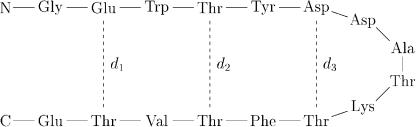
Figure 51. A schematic of Protein G (41–56) in its hairpin conformation. The dotted lines indicate hydrogen bonds, and the distances d1; d2, and d3 refer to the distances between the Ca atoms.

the Effective Energy Function (EEF1) [165], which is the CHARMM potential plus a solvation term based on a Gaussian solvent exclusion model.

Segment 41–56 of Protein G is a 16-residue peptide that has been determined experimentally to fold into a b-hairpin in aqueous solution [135]. A schematic of this hairpin structure is depicted in Fig. 51. The hairpin structure is stabilized by the formation of three pairs of hydrogen bonds as indicated in Fig. 51. The corresponding distances between the Ca atoms are designated d1, d2, and d3 and will play an important role in our analysis of this molecule.

The potential energy surface we employ for this peptide in aqueous solution is split into two terms:

E ¼ Epep þ Esolv

where Epep includes the peptide intramolecular interactions, and Esolv includes the peptide–solvent and solvent–solvent interactions.

The intramolecular interaction term, Epep, is modeled with the CHARMM22 potential energy function, an all-atom potential that takes the general form [32,166]

Epep ¼ X Kbðb b0Þ2 þ

X

KUBðS S0Þ2 þ

X Kyðy y0Þ2

bonds

Urey Bradley

angles

þ

X

Kf

1

þ

cos

nf

d

X Ko

o

o0

Þ

2

dihedrals

ð

ð

ÞÞ þ improper

ð

dihedrals

þ

X nEij½ðRijmin=rijÞ12 2ðRijmin=rijÞ6& þ ðqiqjÞ=rijo

ð99Þ

nonbond

The quantities b, S, y, f, o are the bond length, Urey–Bradley distance, bond angle, dihedral angle, and improper dihedral angle, respectively, with the zero subscript representing equilibrium values. The parameters have been determined empirically and are given in Ref. [166].

deterministic global optimization and ab initio approaches 405

The solvation term, Esolv, is based on the Gaussian solvent exclusion model,

which takes the general form [165]

X

Esolv ¼	i	Gisolv
		(	ref		aie ððrij RiÞ=liÞ2		)
¼	X		Gi	X		Vi	ð	100	Þ
					2
	i				4prij
				j¼6 i

where rij is the distance between atoms i and j. The parameters Gref , ai, Ri, li, and Vi can be found in Ref. [165]. In addition, partial charges for several atoms in charged residues have been modified, effectively neutralizing the side chains in the CHARMM22 potential.

To simplify calculations, we fix the bond lengths and bond angles to their equilibrium values according to the CHARMM22 parameters, allowing only the f, c, o, and w dihedral angles to vary. This reduces the number of degrees of freedom from 3Na 6 ¼ 735 to Nh ¼ 88. Energy values, as well as the Cartesian gradient and Hessian matrix, were computed by the TINKER software package [167]. The Cartesian gradients and Hessians were converted to torsional gradients and Hessians by methods developed in our computer lab. All in all, one Hessian evaluation requires approximately 0:50 sec of CPU time on a 600-MHz pentium machine running linux, where the bulk of the calculations were performed.

In order to study the folding pathways of Protein G (41–56), we need to generate an adequate sample of stationary points of the potential energy surface. Not only do we need to generate conformations that resemble the hairpin native state, as well as extended conformations, but we also need to find conformations that lie along the low-lying pathways connecting these two regions of conformation space. Thus, we need to find low-lying conformations, as well as transition states, over a large region of conformation space.

The approach we have chosen to follow is to first generate an initial sampling of minima, forming a ‘‘scaffolding,’’ and then building upon that scaffolding by performing uphill and downhill searches using an eigenmode-following algorithm. Before carrying out this search, however, we first want to identify the global minimum energy conformation on the potential energy surface, which will serve as the native structure. The results of the global minimum search are given in Fig. 52. The study of the pathways for the transitions from extended to b-sheet conformations is currently in progress.

V.PROTEIN–PROTEIN INTERACTIONS

Understanding protein–protein interactions, also known as peptide docking, is critically important for rational protein engineering and pharmaceutical design.