Enzymes (Second Edition)

320 TIME-DEPENDENT INHIBITION

binder, it is said to be a slow, tight binding inhibitor, and the depletion of the free enzyme and free inhibitor concentrations due to formation of the EI complex also must be taken into account:

K	([E ] [EI])([I] [EI])	(10.2)
	EI

where [E ] represents the concentration of total enzyme (i.e., in all forms) present in solution.

In Scheme C, the enzyme encounters the inhibitor and establishes a binding equilibrium that is defined by the on and off rate constants k and k , just as in Scheme B. In Scheme C, however, the binding of the inhibitor induces in the enzyme a conformational transition, or isomerization, that leads to a new enzyme—inhibitor complex E*I; the forward and reverse rate constants for the equilibrium between these two inhibitor-bound conformations of the enzyme

are given by k and k , respectively. The dissociation constant for the initial EI
complex is still given by K	(i.e., k /k ), but a second dissociation constant for
the second enzyme conformation K* must be considered as well. This second
dissociation constant is given by:
K*		K k		[E][I]		(10.3)
		k k		[EI] [E*I]
To observe a slow onset of inhibition, K* must be much less than K						. Hence,
in this situation, the isomerization of the enzyme leads to much tighter binding

between the enzyme and the inhibitor. As with Scheme B, if the inhibitor is of the slow, tight binding variety, the diminution of free enzyme and free inhibitor must be explicitly accounted for in the expressions for both K and K* (see Morrison and Walsh, 1988).

Note that to observe slow binding kinetics it is not sufficient for the conversion of EI to E*I alone to be slow. The reverse reaction must be slow as well. In fact, for the slow binding to be detected, the reverse rate constant

(k ) must be less than the forward isomerization rate (k ). In the extreme case

(k k ), one does not observe a measurable return to the EI conformation and the enzyme isomerization step will appear to lead to irreversible inhibition. Under these conditions, k can be considered to be insignificant, and the isomerization can be treated practically as an irreversible step dominated by the rate constant k .

Finally, in Scheme D we consider two modes of interaction of the inhibitor with the enzyme for which k is truly equal to zero; that is, we are dealing with irreversible enzyme inactivation. We must make the distinction here between reversible and irreversible inhibition. In all the inhibitory schemes we have considered thus far, even in the case of slow tight binding inhibition, k has been nonzero. This rate constant may be very small, and the inhibitors may act, for all practical purposes, as irreversible. With enough dilution of the EI complex and enough time, however, one can eventually recover an active free

PROGRESS CURVES FOR SLOW BINDING INHIBITORS

321

enzyme population. In the case of an irreversible inhibitor, the enzyme molecule that has bound the inhibitor is permanently incapacitated. No amount of time or dilution will result in a reactivation of the enzyme that has encountered inhibitors of these types. Such inhibitors hence are often referred to as enzyme inactivators.

The first example of irreversible inhibition is the process known as affinity labeling or covalent modification of the enzyme. In this case, the inhibitory compound binds to the enzyme and covalently modifies a catalytically essential residue or residues on the enzyme. The covalent modification involves some chemical alteration of the inhibitory molecule, but the process is based on chemistry that occurs at the modification site in the absence of any enzymecatalyzed reaction. Affinity labels are useful not only as inhibitors of enzyme activity; they also have become valuable research tools. Some of these compounds are very selective for specific amino acid residues and can thus be used to identify key residues involved in the catalytic cycle of the enzyme. See Section 10.5.3 and Lundblad (1991), and Copeland (1994).

In the second form of irreversible inactivation we shall consider, mechanismbased inhibition, the inhibitory molecule binds to the enzyme active site and is recognized by the enzyme as a substrate analogue. The inhibitor is therefore chemically transformed through the catalytic mechanism of the enzyme to form an E—I complex that can no longer function catalytically. Many of these inhibitors inactivate the enzyme by forming an irreversible covalent E—I adduct. In other cases, the inhibitory molecule is subsequently released from the enzyme (a process referred to as noncovalent inactivation), but the enzyme has been permanently trapped in a form that can no longer support catalysis. Because they are chemically altered via the mechanism of enzymatic catalysis at the active site, mechanism-based inhibitors always act as competitive enzyme inactivators. These inhibitors have been referred to by a variety of names in the literature: suicide substrates, suicide enzyme inactivators, k

inhibitors, enzyme-activated irreversible inhibitors, Trojan horse inactivators, enzyme-induced inactivators, dynamic affinity labels, trap substrates, and so on (Silverman, 1988a).

In the discussion that follows we shall describe experimental methods for detecting the time dependence of slow binding inhibitors, and data analysis methods that allow us to distinguish among the different potential modes of interaction with the enzyme. We shall also discuss the appropriate determination of the inhibitor constants K and K* for these inhibitors.

10.1 PROGRESS CURVES FOR SLOW BINDING INHIBITORS

The progress curves for an enzyme reaction in the presence of a slow binding inhibitor will not display the simple linear product-versus-time relationship we have seen for simple reversible inhibitors. Rather, product formation over time will be a curvilinear function because of the slow onset of inhibition for these

322 TIME-DEPENDENT INHIBITION

Figure 10.2 Examples of progress curves in the presence of varying concentrations of a time-dependent enzyme inhibitor for a reaction initiated by adding enzyme to a mixture containing substrate and inhibitor. Curves are numbered to indicate the relative concentrations of inhibitor present. Note that over the entire 10-minute time window, the uninhibited enzyme displays a linear progress curve.

compounds. Figure 10.2 illustrates typical progress curves for a slow binding inhibitor when the enzymatic reaction is initiated by addition of enzyme. Over a time period in which the uninhibited enzyme displays a simple linear progress curve, the data in the presence of the slow binding inhibitor will display a quasi-linear relationship with time in the early part of the curve, converting later to a different (slower) linear relationship between product and time. Note that it is critical to establish a time window covering the linear portion of the uninhibited reaction progress curve, during which one can observe the change in slope that occurs with inhibition. If the onset of inhibition is very slow, a long time window may be required to observe the changes illustrated in Figure 10.2. With long time windows, however, one runs the risk of reaching significant substrate depletion, which would invalidate the subsequent data analysis. Thus it may be necessary to evaluate several combinations of enzyme, substrate, and inhibitor concentrations to find an appropriate range of each for conducting time-dependent measurements. With these cautions addressed, the progress curves at different inhibitor concentrations can be described by Equation 10.4:

[P] v t	v	v	[1 exp( k t)]	(10.4)
	k

PROGRESS CURVES FOR SLOW BINDING INHIBITORS

323

where v and v are the initial and steady state (i.e., final) velocities of the reaction in the presence of inhibitor, k is the apparent first-order rate constant for the interconversion between v and v , and t is time.

Morrison and Walsh (1988) have provided explicit mathematical expressions for v and v in the case of a competitive slow binding inhibitor, illustrating that v and v are functions (similar to Equation 8.10) of V , [S], K , and either K or K* (for inhibitors that act according to Scheme C in Figure 10.1), respectively. For our purposes, it is sufficient to treat Equation 10.4 as an empirical equation that makes possible the extraction from the experimental data of values for v , v , and most importantly, k . Note that v may or may not vary with inhibitor concentration, depending on the relative values of K and K*, and the ratio of [I] to K (Morrison and Walsh, 1988). The value of v will be a finite, nonzero value as long as the inhibitor is not an irreversible enzyme inactivator. In the latter case, the value of v will eventually reach zero.

A second strategy for measuring progress curves for slow binding inhibitors is to preincubate the enzyme with the inhibitor for a long time period relative to the rate of inhibitor binding, and to then initiate the reaction by diluting the enzyme—inhibitor solution with a solution containing the substrate for the enzyme. During the preincubation period the equilibria between enzyme and inhibitor are established, and addition of substrate perturbs this equilibrium. Because of the slow off rate of the inhibitor, the progress curve will display an initial shallow slope, which eventually turns over to the steady state velocity, as illustrated in Figure 10.3. The progress curves seen here also are well described by Equation 10.4, except that now the initial velocity is lower than the steady state velocity, whereas for data obtained by initiating the reaction with enzyme, the initial velocity is greater than the steady state velocity. To highlight this difference, some authors replace the term v in Equation 10.4 with v in the case of reactions initiated with substrate. Morrison and Walsh (1988) again provide an explicit mathematical form for v , which depends on the V , [S], K , [I], K , K*, and the volume ratio between the preincubation enzyme—inhibitor solution and the final volume of the total reaction mixture. Again, for our purposes we can use Equation 10.4 as an empirical equation, allowing v (or v ), v , and k to be adjustable parameters whose values are determined by nonlinear curve-fitting analysis.

Inhibitors that are very tight binding, as well as time dependent, almost always conform to Scheme C of Figure 10.1 (Morrison and Walsh, 1988). In this case the progress curves also will be influenced by the depletion of the free enzyme and free inhibitor populations that occurs. To account for these diminished populations, Equation 10.4 must be modified as follows:

[P] v t	(v		v )(1 )		ln		[1 exp( k t)]		(10.5)
			k				1

324 TIME-DEPENDENT INHIBITION

Figure 10.3 Examples of progress curves in the presence of varying concentrations of a time-dependent enzyme inhibitor for a reaction initiated by diluting an enzyme—inhibitor complex into the reaction buffer containing substrate. Curves are numbered to indicate the relative concentrations of inhibitor.

where is given by
K* [E ] [I ] Q					[E ]		v
							1			(10.6)
	K* [E ] [I ] Q				[I ]			v

where

Q [(K* [I ] [E ]) 4(K* [E ])] (K* [I ] [E ]) (10.7)

Throughout Equations 10.5—10.7, [E ] and [I ] refer to the total concentrations (i.e., all forms) of enzyme and inhibitor, respectively. Further discussion of the data analysis for slow, very tight binding inhibitors can be found in the review by Morrison and Walsh (1988).

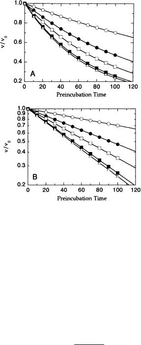
If inhibitor binding (or release) is very slow compared to the rate of uninhibited enzyme turnover, another convenient experimental strategy can be employed to determine k . Essentially, the enzyme is preincubated with the inhibitor for different lengths of time before the steady state velocity of the reaction is measured. For example, if the steady state velocity of the reaction can be measured over a 30-second time window, but the inhibitor binding event occurs over the course of tens of minutes, the enzyme could be

DISTINGUISHING BETWEEN SLOW BINDING SCHEMES

325

preincubated with the inhibitor between 0 and 120 minutes in 5-minute intervals, and the velocity of the reaction measured after each of the different preincubation times. Figure 10.4 illustrates the type of data this treatment would produce. For a fixed inhibitor concentration, the fractional velocity remaining after a given preincubation time will fall off according to Equation 10.8:

v

exp( k t)

(10.8)

v

Therefore, at a fixed inhibitor concentration, the fractional velocity will decay exponentially with preincubation time, as in Figure 10.4A. For convenience, we can recast Equation 10.8 by taking the logarithm of each side to obtain a linear function:

2.303 log	v	k t	(10.9)
	v

Thus the value of k at a fixed inhibitor concentration can be determined directly from the slope of a semilog plot of fractional velocity as a function of preincubation time, as in Figure 10.4B.

10.2 DISTINGUISHING BETWEEN SLOW BINDING SCHEMES

To distinguish among the schemes illustrated in Figure 10.1, one must determine the effect of inhibitor concentration on the apparent first-order rate constant k . We shall present the relationships between k and [I] for these various schemes without deriving them explicitly. A full treatment of the derivation of these equations can be found in Morrison and Walsh (1988) and references therein.

10.2.1 Scheme B

For an inhibitor that binds according to Scheme B of Figure 10.1, the relationship between k and [I] is given by Equation 10.10:

					K
k	k		1		[I]		(10.10)

where K is the apparent K , which is related to the true K by different functions depending on the mode of inhibitor interaction with the enzyme (i.e., competitive, noncompetitive, uncompetitive, etc.; see Section 10.3). From Equation 10.10 we see that a plot of k as a function of [I] should yield a straight line with slope equal to k /K and y intercept equal to k (Figure 10.5). Thus from linear regression analysis of such data, one can simultaneously

326 TIME-DEPENDENT INHIBITION

Figure 10.4 Preincubation time dependence of the fractional velocity of an enzyme-catalyzed reaction in the presence of varying concentrations of a slow binding inhibitor: data on a linear scale (A) and on a semilog scale (B).

determine the values of k and K . If the inhibitor modality is known, K

can be converted into K (Section 10.3), and from this the value of k can be determined by means of Equation 10.1.

10.2.2 Scheme C

For inhibitors corresponding to Scheme C of Figure 10.1, k is related to [I] as follows:

			k [I]
k	k				(10.11)
			K [I]

DISTINGUISHING BETWEEN SLOW BINDING SCHEMES

327

Figure 10.5 Plot of k as a function of inhibitor concentration for a slow binding inhibitor that conforms to Scheme B of Figure 10.1.

which can be recast thus:
1			[I]
		K*
k k 1			[I]				(10.12)
			K
The form of Equations 10.11 and 10.12 predicts that k							will vary as a
hyperbolic function of [I], as illustrated in Figure 10.6. The y intercept of the

curve in this figure provides an estimate of the rate constant k , while the
maximum value of k		expected at infinite inhibitor concentration according
to Equation 10.11, is k		k . Hence, by nonlinear curve fitting of the data to
Equation 10.11 one can simultaneously determine the values of k , K , and
K* .
Note that if K were much greater than K*, the concentrations of inhibitor
required for slow	binding inhibition would be much less than K . Under these
circumstances, the steady state concentration of [EI] would be kinetically
insignificant, and Equation 10.11 would thus reduce to:

					K
k	k			1	[I]		(10.13)
					*

Thus for this situation a plot of k as function of [I] would again yield a straight-line relationship, as we saw for inhibitors associated with Scheme B. In fact, when a straight-line relationship is observed in the plot of k versus [I], one cannot readily distinguish between these two situations.

328 TIME-DEPENDENT INHIBITION

Figure 10.6 Plot of k as a function of inhibitor concentration for a slow binding inhibitor that conforms to Scheme C of Figure 10.1.

10.2.3 Scheme D

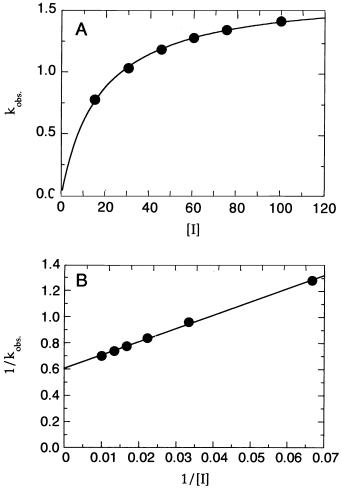
If the kinetic constant k is very small in Scheme C, or zero as in Scheme D, the inhibitor acts, for all practical purposes, as an irreversible inactivator of the enzyme. In such cases, Equation 10.11 reduces to:

k [I]

k (10.14)

K [I]

Here again, a plot of k as a function of [I] will yield a hyperbolic curve (Figure 10.7A), but now the y intercept will be zero (reflecting the zero, or near-zero, value of k ).

For irreversible inhibitors, the return to free E and free I from the EI complex is greatly perturbed by the irreversibility of the subsequent inactivation event (represented by k ). For this reason, Tipton (1973) and Kitz and Wilson (1962) make the point that for irreversible inactivators, the term K no longer represents the simple dissociation constant for the EI complex. Rather, the term K in Equation 10.14 is defined as the apparent concentration of inhibitor required to reach half-maximal rate of inactivation of the enzyme.

Kitz and Wilson (1962) also replace k in Equation 10.14 with k , which they define as the maximal rate of enzyme inactivation. With these definitions,

the parameters k and K are reminiscent of the parameters V and K , respectively, from the Henri—Michaelis—Menten equation (Chapter 5). Just as

DISTINGUISHING BETWEEN SLOW BINDING SCHEMES

329

Figure 10.7 (A) Plot of k as a function of inhibitor concentration for a slow binding inhibitor that conforms to Scheme D of Figure 10.1. (B) The data as in (A) presented as a doublereciprocal plot. The nonzero intercept indicates that the inactivation proceeds through a two-step mechanism: an initial binding step followed by a slower inactivation event.

the ratio k /K is the best measure of the catalytic efficiency of an enzymecatalyzed reaction, the best measure of inhibitory potency for an irreversible

inhibitor is the second-order rate constant obtained from the ratio k /K . Similar to the Lineweaver—Burk plots encountered in Chapter 5, a double-

reciprocal plot of 1/k as a function of 1/[I] yields a straight-line relationship. Most irreversible inhibitors bind to the enzyme active site in a reversible manner (represented by K ) before the slower inactivation event (represented by k ) proceeds. Thus, as illustrated by Scheme D in Figure 10.1, the