1Foundation of Mathematical Biology / Foundation of Mathematical Biology

UCSF

Bad news: the correlations appear to be no better than chance at p = 0.05

We compute the direct correlation for each of

1225 loci

♦Strongest correlation at 8q24

♦Many other peaks

Compute level of significance using permutation analysis

We get a critical value of

0.36

Correlation Magnitude

Correlation magnitude with overall survival

0.35

0.3

0.25

0.2

0.15

0.1

0.05

0

1

2

3

4

5

6

7

8

9

10

11

12

13

14

15

16

17

18

19 20 2122 X

Genomic Position

Cumulative Histogram of Correlation Magnitudes

	1
	0.9
	0.8
	0.7						p = 0.05
Proportion							threshold
	0.6						is 0.36
	0.5
Cumulative
	0.4
	0.3
	0.2
	0.1
	0
	0.15	0.2	0.25	0.3	0.35	0.4	0.45	0.5

Correlation Magnitude

UCSF

General Principle: Reduce the number of observations

Any method we can use to subselect a smaller set of observations from the larger set helps us, provided:

♦The subselection method must be orthogonal to the correlation being studied

•If we’re trying to link copy number to survival, we can’t systematically employ the survival outcomes in making our subselection

♦Ideally, the method should have some compelling intuitive support based on the data

♦Restricting observations based on frequency/magnitude is a generally useful technique: it tends to eliminate noise

UCSF

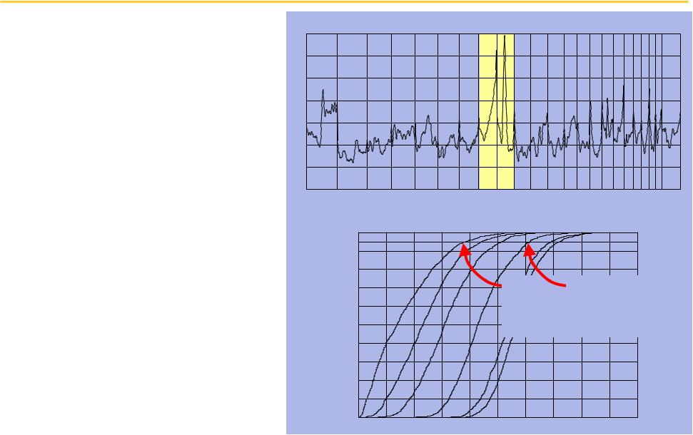
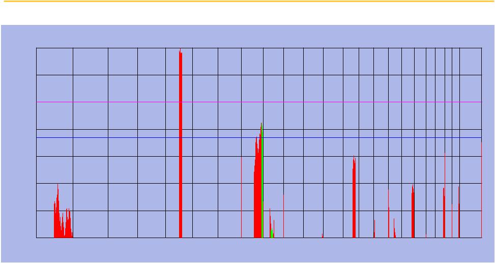
By including frequency and amplitude, we can detect weaker correlations

The magnitude of copy number variation is not uniformly distributed

♦9q13 has the largest cumulative variation

♦8q24 has the next highest

Significance thresholds on correlation vary with

“energy”

♦Energy 0.0, t = 0.36

♦Energy 3.0, t = 0.31

♦Energy 6.0, t = 0.19

							CGH variation energy
7
6
5
4
Energy
3
2
1
0
1	2	3	4	5	6	7	8	9	10	11	12	13	14	15	16	17	18	19 20 2122 X
							Genomic Position
			Cumulative Histogram of Correlation Magnitudes with Multiple Energies
		1
		0.9
		0.8
		0.7							E = 6.0,				E = 3.0,
	Proportion	0.6							p = 0.05				p = 0.05
									threshold				threshold
		0.5							is 0.19				is 0.31
	Cumulative
		0.4
		0.3
		0.2
		0.1
		0
		0	0.05	0.1	0.15		0.2	0.25		0.3	0.35		0.4		0.45			0.5
							Correlation Magnitude

UCSF

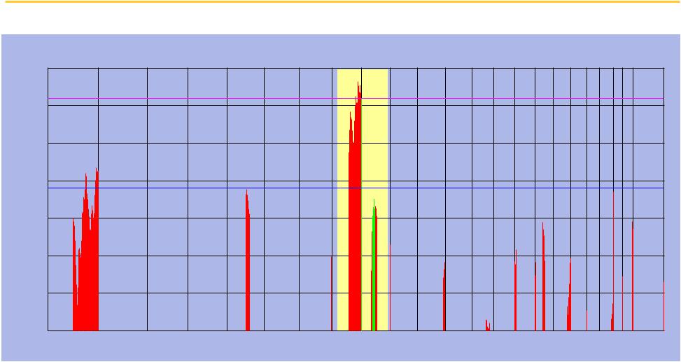
Both 8q24 and 9q13 are significantly correlated with survival

Correlation Magnitude

Correlation Magnitude with Overall Survival

0.35

0.3

0.25

0.2

0.15

0.1

0.05

0

1

2

3

4

5

6

7

8

9

10

11

12

13

14

15

16

17

18

19 20 2122 X

Genomic Position

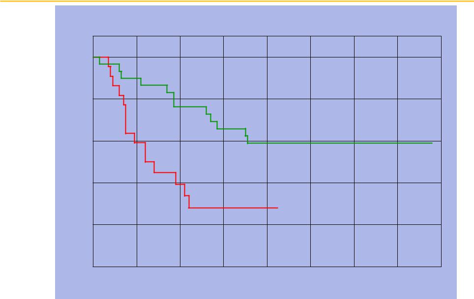
UCSF Amplification at 8q24: poorer survival (p < 0.01)

Kaplan-Meier Plot of Normal vs Amplified at 8q24

Fraction Surviving

1

0.8

Normal

0.6

0.4

Amplified

0.2

0

0

20

40

60

80

100

120

140

160

Survival Duration

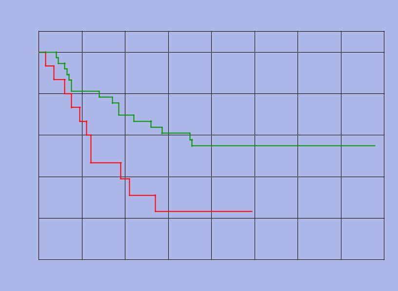
UCSF		Deletion at 9q13: poorer survival (p < 0.01)
		Kaplan-Meier Plot of Normal vs Deleted at 9q13

Fraction Surviving

1

0.8

0.6	Normal

0.4

Deleted

0.2

0

0

20

40

60

80

100

120

140

160

Survival Duration

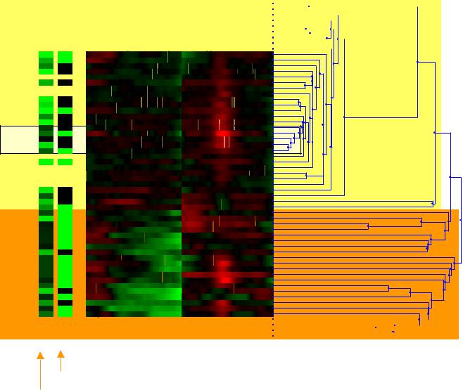
UCSF		Clustering based on chromosomes 8 and 9 reveal
		patterns of survival and tumor phenotype

Cluster profiles based on Chr 8,9

♦Display raw data

♦Display survival, p53 status

Cluster enrichment is statistically significant

♦Orange block

•Surv < 35 months

•p53 often mutant

♦Yellow block

•Surv > 75 months

•p53 often wt

MT64_mt:

MT67_wt:

N14

MT160_mt:

MT101_mt:

MT221_wt:

N11

N28

MT264_wt:

N16

MT46_wt:

N26

N31

107B_mt:

MT60_wt:

MT132_mt:
MT24_mt:			N30	N39
MT54_wt:
MT21_wt:		N22
012.10-NOR:		N18
MT5_wt:		N17
125.10-NOR:		N9N21
020.10-NOR:			N29
MT17_wt:		N3
MT44_wt:			N25
		N5 N20
MT3_mt:
MT18_wt:		N15		N32
MT19_wt:		N10N7	N23
406A_wt:		N6
				N49
123B_mt:		N4
406B_wt:	N2 N8
MT31_wt:	N1	N13N19	N27
MT65_mt:	N0
			N24
011.10-NOR:
MT181_mt:
017.10-NOR:
035.10-NOR:		N12			N55
012.20-NOR:
016.10-NOR:
MT38_wt:
MT57_wt:
MT43_wt:				N48
MT20_mt:
MT418_mt:
MT59_mt:				N41	N53 N58
309A_mt:
UT274_mt:				N33	N52
MT112_mt:
				N46
MT161_mt:
208A_mt:				N44
MT51_wt:				N42
UT250_mt:
UT065_mt:					N57
UT252_mt:					N56
101A_mt:					N54
UT009_mt:					N51
405A_mt:				N35
					N50
MT49_wt:
				N38
UT164_mt:				N47
MT209_wt:
111A_mt:				N45
MT29_mt:				N43

214A_wt:

N40

MT61_wt:

N34

N37

MT342_wt:

N36

111B_mt:

sv

p53

chr8-9

p53 status (green = mut, black = wt) Survival (black = low, green = high)

UCSF

Deletion at 5q11-31 and amplification at 8q24 are correlated with mutant p53

Correlation Magnitude

Correlation magnitude with p53 status

0.35

0.3

0.25

0.2

0.15

0.1

0.05

0

1

2

3

4

5

6

7

8

9

10

11

12

13

14

15

16

17

18

19 20 2122 X

Genomic Position

Some genes on 5q: APC and IL3

UCSF

Conclusions on permutation and resampling methods

Permutation and resampling methods offer a means to replace complex assumptions with counting.

We can generalize the concept of a statistic to any computable value and apply permutation methods to judge significance.

This can be directly applied in addressing the problem of multiple testing in array-based data.

If we can reduce the number of tests based on an orthogonal observation, we gain statistical power.

Further reading

♦Resampling-Based Multiple Testing : Examples and Methods for P-Value Adjustment by Peter H. Westfall, S. Stanley Young

♦Jain AN, Chin K, Borresen-Dale AL, Erikstein BK, Eynstein Lonning P, Kaaresen R, Gray JW. Quantitative analysis of chromosomal CGH in human breast tumors associates copy number abnormalities with p53 status and patient survival.Proc Natl Acad Sci U S A. 2001 Jul 3;98(14):7952-7.

♦Dudoit, S., Yang, Y.H., Callow, M.J., and Speed, T. (2000) Statistical methods for identifying differentially expressed genes. Unpublished (Berkeley Stat Dept. Technical Report #578). (To appear: JASA)

♦Tusher V, Tibshirani R, and Chu G. (2001) Significance analysis of microarrays applied to the ionizing radiation response. PNAS 98: 5116-5124.

UCSF

So how do we design array-based experiments?

General scheme

♦Use P samples to screen large number of variables (N) to select a much smaller number (M)

•Expectation, despite multiple comparisons, is that the highest ranked variables contain true effects if they exist

•We must pick M such that for a particular effect size, it is very likely that our M will include a true effect of the specified size

♦On K new samples, screen the M variables in order to identify the true effects with reasonable power

So how do we pick P, N, M, and K?

♦Pick N based on experimental considerations: What pool of variables do you need to consider?

♦Pick P based on practical considerations: you probably won’t be able to pick P large enough to get adequate power.

♦Pick M such that, with preliminary data, the null distribution of the Mth strongest effect makes it very likely that if an effect of the size you want exists, it will be within the top M.

♦Now choose K such that with M variables, you have adequate power to see an effect of the size you want to find.

So how do you choose an effect size?

♦Based on what is of practical significance

♦Note: you can play with the effect size to modulate your power. This is a nasty business though.