

Contents
1 Introduction . . . . . . . . . . . . . . . . . . . . . . . . . . . . . . . . . . . . . . . . . . . . . . |
1 |
||
1.1 |
Historical Survey . . . . . . . . . . . . . . . . . . . . . . . . . . . . . . . . . . . . . . . |
2 |
|
1.2 |
Patterns in Nonlinear Optical Resonators . . . . . . . . . . . . . . . . . . |
4 |
|
|
1.2.1 Localized Structures: Vortices and Solitons . . . . . . . . . . |
6 |
|
|
1.2.2 |
Extended Patterns . . . . . . . . . . . . . . . . . . . . . . . . . . . . . . . |
8 |
1.3 |
Optical Patterns in Other Configurations . . . . . . . . . . . . . . . . . . |
11 |
|
|
1.3.1 |
Mirrorless Configuration . . . . . . . . . . . . . . . . . . . . . . . . . . |
11 |
|
1.3.2 |
Single-Feedback-Mirror Configuration . . . . . . . . . . . . . . . |
12 |
|
1.3.3 |
Optical Feedback Loops . . . . . . . . . . . . . . . . . . . . . . . . . . . |
12 |
1.4 |
The Contents of this Book . . . . . . . . . . . . . . . . . . . . . . . . . . . . . . . |
15 |
|
References |
. . . . . . . . . . . . . . . . . . . . . . . . . . . . . . . . . . . . . . . . . . . . . . . . . |
19 |
|
2 Order Parameter Equations for Lasers . . . . . . . . . . . . . . . . . . . . 33 2.1 Model of a Laser . . . . . . . . . . . . . . . . . . . . . . . . . . . . . . . . . . . . . . . 34 2.2 Linear Stability Analysis . . . . . . . . . . . . . . . . . . . . . . . . . . . . . . . . 36 2.3 Derivation of the Laser Order Parameter Equation. . . . . . . . . . 41 2.3.1 Adiabatic Elimination . . . . . . . . . . . . . . . . . . . . . . . . . . . . 41 2.3.2 Multiple-Scale Expansion. . . . . . . . . . . . . . . . . . . . . . . . . . 46 References . . . . . . . . . . . . . . . . . . . . . . . . . . . . . . . . . . . . . . . . . . . . . . . . . 48
3Order Parameter Equations
for Other Nonlinear Resonators . . . . . . . . . . . . . . . . . . . . . . . . . . |
51 |
||
3.1 |
Optical Parametric Oscillators . . . . . . . . . . . . . . . . . . . . . . . . . . . |
51 |
|
3.2 |
The Real Swift–Hohenberg Equation for DOPOs . . . . . . . . . . . |
52 |
|
|
3.2.1 |
Linear Stability Analysis . . . . . . . . . . . . . . . . . . . . . . . . . . |
52 |
|
3.2.2 |
Scales . . . . . . . . . . . . . . . . . . . . . . . . . . . . . . . . . . . . . . . . . . . |
53 |
|
3.2.3 Derivation of the OPE . . . . . . . . . . . . . . . . . . . . . . . . . . . . |
54 |
|
3.3 |
The Complex Swift–Hohenberg Equation for OPOs . . . . . . . . . |
55 |
|
|
3.3.1 |
Linear Stability Analysis . . . . . . . . . . . . . . . . . . . . . . . . . . |
56 |
|
3.3.2 |
Scales . . . . . . . . . . . . . . . . . . . . . . . . . . . . . . . . . . . . . . . . . . . |
57 |
|
3.3.3 Derivation of the OPE . . . . . . . . . . . . . . . . . . . . . . . . . . . . |
57 |
|
3.4 |
The |
Order Parameter Equation |
|
|
for Photorefractive Oscillators. . . . . . . . . . . . . . . . . . . . . . . . . . . . |
59 |
|
|
3.4.1 |
Description and Model . . . . . . . . . . . . . . . . . . . . . . . . . . . . |
59 |
|
3.4.2 Adiabatic Elimination and Operator Inversion . . . . . . . |
60 |
|
XContents
3.5Phenomenological Derivation
of Order Parameter Equations . . . . . . . . . . . . . . . . . . . . . . . . . . . 61
References . . . . . . . . . . . . . . . . . . . . . . . . . . . . . . . . . . . . . . . . . . . . . . . . . 63
4Zero Detuning: Laser Hydrodynamics
and Optical Vortices . . . . . . . . . . . . . . . . . . . . . . . . . . . . . . . . . . . . . . 65
4.1 Hydrodynamic Form . . . . . . . . . . . . . . . . . . . . . . . . . . . . . . . . . . . . 65
4.2 Optical Vortices . . . . . . . . . . . . . . . . . . . . . . . . . . . . . . . . . . . . . . . . 67
4.2.1 Strong Di raction . . . . . . . . . . . . . . . . . . . . . . . . . . . . . . . . 68
4.2.2 Strong Di usion. . . . . . . . . . . . . . . . . . . . . . . . . . . . . . . . . . 71
4.2.3 Intermediate Cases . . . . . . . . . . . . . . . . . . . . . . . . . . . . . . . 72
4.3 Vortex Interactions . . . . . . . . . . . . . . . . . . . . . . . . . . . . . . . . . . . . . 74
References . . . . . . . . . . . . . . . . . . . . . . . . . . . . . . . . . . . . . . . . . . . . . . . . . 79
5Finite Detuning: Vortex Sheets
and Vortex Lattices. . . . . . . . . . . . . . . . . . . . . . . . . . . . . . . . . . . . . . . 81 5.1 Vortices “Riding” on Tilted Waves. . . . . . . . . . . . . . . . . . . . . . . . 82 5.2 Domains of Tilted Waves . . . . . . . . . . . . . . . . . . . . . . . . . . . . . . . . 84 5.3 Square Vortex Lattices . . . . . . . . . . . . . . . . . . . . . . . . . . . . . . . . . . 87
References . . . . . . . . . . . . . . . . . . . . . . . . . . . . . . . . . . . . . . . . . . . . . . . . . 90
6 Resonators with Curved Mirrors. . . . . . . . . . . . . . . . . . . . . . . . . . 91 6.1 Weakly Curved Mirrors . . . . . . . . . . . . . . . . . . . . . . . . . . . . . . . . . 92 6.2 Mode Expansion . . . . . . . . . . . . . . . . . . . . . . . . . . . . . . . . . . . . . . . 93 6.2.1 Circling Vortices . . . . . . . . . . . . . . . . . . . . . . . . . . . . . . . . . 94 6.2.2 Locking of Transverse Modes . . . . . . . . . . . . . . . . . . . . . . 95 6.3 Degenerate Resonators . . . . . . . . . . . . . . . . . . . . . . . . . . . . . . . . . . 97
References . . . . . . . . . . . . . . . . . . . . . . . . . . . . . . . . . . . . . . . . . . . . . . . . . 102
7 The Restless Vortex . . . . . . . . . . . . . . . . . . . . . . . . . . . . . . . . . . . . . . 103 7.1 The Model . . . . . . . . . . . . . . . . . . . . . . . . . . . . . . . . . . . . . . . . . . . . 103 7.2 Single Vortex . . . . . . . . . . . . . . . . . . . . . . . . . . . . . . . . . . . . . . . . . . 105 7.3 Vortex Lattices. . . . . . . . . . . . . . . . . . . . . . . . . . . . . . . . . . . . . . . . . 108 7.3.1 “Optical” Oscillation Mode . . . . . . . . . . . . . . . . . . . . . . . . 109 7.3.2 Parallel translation of a vortex lattice . . . . . . . . . . . . . . . 110 7.4 Experimental Demonstration of the “Restless” Vortex . . . . . . . 111 7.4.1 Mode Expansion . . . . . . . . . . . . . . . . . . . . . . . . . . . . . . . . . 111 7.4.2 Phase-Insensitive Modes. . . . . . . . . . . . . . . . . . . . . . . . . . . 113 7.4.3 Phase-Sensitive Modes . . . . . . . . . . . . . . . . . . . . . . . . . . . . 114
References . . . . . . . . . . . . . . . . . . . . . . . . . . . . . . . . . . . . . . . . . . . . . . . . . 115
8 Domains and Spatial Solitons . . . . . . . . . . . . . . . . . . . . . . . . . . . . . 117
8.1 Subcritical Versus Supercritical Systems . . . . . . . . . . . . . . . . . . . 117
8.2 Mechanisms Allowing Soliton Formation. . . . . . . . . . . . . . . . . . . 118
8.2.1 Supercritical Hopf Bifurcation . . . . . . . . . . . . . . . . . . . . . 119
Contents XI
8.2.2 Subcritical Hopf Bifurcation . . . . . . . . . . . . . . . . . . . . . . . 120
8.3 Amplitude and Phase Domains . . . . . . . . . . . . . . . . . . . . . . . . . . . 122
8.4 Amplitude and Phase Spatial Solitons . . . . . . . . . . . . . . . . . . . . . 123
References . . . . . . . . . . . . . . . . . . . . . . . . . . . . . . . . . . . . . . . . . . . . . . . . . 124
9 Subcritical Solitons I: Saturable Absorber . . . . . . . . . . . . . . . . 125
9.1 Model and Order Parameter Equation . . . . . . . . . . . . . . . . . . . . 125
9.2 Amplitude Domains and Spatial Solitons . . . . . . . . . . . . . . . . . . 127
9.3 Numerical Simulations . . . . . . . . . . . . . . . . . . . . . . . . . . . . . . . . . . 129
9.3.1 Soliton Formation . . . . . . . . . . . . . . . . . . . . . . . . . . . . . . . . 129
9.3.2 Soliton Manipulation: Positioning, Propagation,
Trapping and Switching . . . . . . . . . . . . . . . . . . . . . . . . . . . 132
9.4 Experiments . . . . . . . . . . . . . . . . . . . . . . . . . . . . . . . . . . . . . . . . . . . 133
References . . . . . . . . . . . . . . . . . . . . . . . . . . . . . . . . . . . . . . . . . . . . . . . . . 138
10 Subcritical Solitons II: |
|
|
Nonlinear Resonance . . . . . . . . . . . . . . . . . . . . . . . . . . . . . . . . . . . . . |
139 |
|
10.1 |
Analysis of the Homogeneous State. |
|
|
Nonlinear Resonance . . . . . . . . . . . . . . . . . . . . . . . . . . . . . . . . . . . . |
139 |
10.2 |
Spatial Solitons . . . . . . . . . . . . . . . . . . . . . . . . . . . . . . . . . . . . . . . . |
141 |
|
10.2.1 One-Dimensional Case . . . . . . . . . . . . . . . . . . . . . . . . . . . . |
141 |
|
10.2.2 Two-Dimensional Case . . . . . . . . . . . . . . . . . . . . . . . . . . . . |
144 |
References . . . . . . . . . . . . . . . . . . . . . . . . . . . . . . . . . . . . . . . . . . . . . . . . . |
146 |
|
11 Phase Domains and Phase Solitons . . . . . . . . . . . . . . . . . . . . . . . 147
11.1 Patterns in Systems with a Real-Valued Order Parameter . . . 147
11.2 Phase Domains. . . . . . . . . . . . . . . . . . . . . . . . . . . . . . . . . . . . . . . . . 148
11.3 Dynamics of Domain Boundaries . . . . . . . . . . . . . . . . . . . . . . . . . 150
11.3.1 Variational Approach . . . . . . . . . . . . . . . . . . . . . . . . . . . . . 150
11.3.2 Two-Dimensional Domains . . . . . . . . . . . . . . . . . . . . . . . . 152
11.4 Phase Solitons . . . . . . . . . . . . . . . . . . . . . . . . . . . . . . . . . . . . . . . . . 155
11.5 Nonmonotonically Decaying Fronts . . . . . . . . . . . . . . . . . . . . . . . 157
11.6 Experimental Realization of Phase Domains
and Solitons . . . . . . . . . . . . . . . . . . . . . . . . . . . . . . . . . . . . . . . . . . . 160
11.7 Domain Boundaries and Image Processing . . . . . . . . . . . . . . . . . 163
References . . . . . . . . . . . . . . . . . . . . . . . . . . . . . . . . . . . . . . . . . . . . . . . . . 166
12 Turing Patterns in Nonlinear Optics . . . . . . . . . . . . . . . . . . . . . . |
169 |
|
12.1 |
The Turing Mechanism in Nonlinear Optics . . . . . . . . . . . . . . . . |
169 |
12.2 |
Laser with Di using Gain . . . . . . . . . . . . . . . . . . . . . . . . . . . . . . . |
171 |
|
12.2.1 General Case . . . . . . . . . . . . . . . . . . . . . . . . . . . . . . . . . . . . |
172 |
|
12.2.2 Laser with Saturable Absorber . . . . . . . . . . . . . . . . . . . . . |
174 |
|
12.2.3 Stabilization of Spatial Solitons by Gain Di usion . . . . |
176 |
12.3 |
Optical Parametric Oscillator |
|
|
with Di racting Pump . . . . . . . . . . . . . . . . . . . . . . . . . . . . . . . . . . |
180 |
XII Contents
12.3.1 Turing Instability in a DOPO . . . . . . . . . . . . . . . . . . . . . . 181 12.3.2 Stochastic Patterns . . . . . . . . . . . . . . . . . . . . . . . . . . . . . . . 184 12.3.3 Spatial Solitons Influenced by Pump Di raction . . . . . . 187 References . . . . . . . . . . . . . . . . . . . . . . . . . . . . . . . . . . . . . . . . . . . . . . . . . 191
13 Three-Dimensional Patterns . . . . . . . . . . . . . . . . . . . . . . . . . . . . . . 193 13.1 The Synchronously Pumped DOPO. . . . . . . . . . . . . . . . . . . . . . . 193 13.1.1 Order Parameter Equation . . . . . . . . . . . . . . . . . . . . . . . . 194 13.2 Patterns Obtained from the 3D Swift–Hohenberg Equation . . 196 13.3 The Nondegenerate OPO . . . . . . . . . . . . . . . . . . . . . . . . . . . . . . . . 200 13.4 Conclusions. . . . . . . . . . . . . . . . . . . . . . . . . . . . . . . . . . . . . . . . . . . . 201 13.4.1 Tunability of a System with a Broad Gain Band. . . . . . 201 13.4.2 Analogy Between 2D and 3D Cases . . . . . . . . . . . . . . . . . 202 References . . . . . . . . . . . . . . . . . . . . . . . . . . . . . . . . . . . . . . . . . . . . . . . . . 202
14 Patterns and Noise . . . . . . . . . . . . . . . . . . . . . . . . . . . . . . . . . . . . . . . 205
14.1 Noise in Condensates . . . . . . . . . . . . . . . . . . . . . . . . . . . . . . . . . . . 206
14.1.1 Spatio-Temporal Noise Spectra . . . . . . . . . . . . . . . . . . . . . 207
14.1.2 Numerical Results . . . . . . . . . . . . . . . . . . . . . . . . . . . . . . . . 210
14.1.3 Consequences . . . . . . . . . . . . . . . . . . . . . . . . . . . . . . . . . . . . 214
14.2 Noisy Stripes . . . . . . . . . . . . . . . . . . . . . . . . . . . . . . . . . . . . . . . . . . 216
14.2.1 Spatio-Temporal Noise Spectra . . . . . . . . . . . . . . . . . . . . . 217
14.2.2 Stochastic Drifts . . . . . . . . . . . . . . . . . . . . . . . . . . . . . . . . . 221
14.2.3 Consequences . . . . . . . . . . . . . . . . . . . . . . . . . . . . . . . . . . . . 223
References . . . . . . . . . . . . . . . . . . . . . . . . . . . . . . . . . . . . . . . . . . . . . . . . . 224
Index . . . . . . . . . . . . . . . . . . . . . . . . . . . . . . . . . . . . . . . . . . . . . . . . . . . . . . . . . 225
1 Introduction
Pattern formation, i.e. the spontaneous emergence of spatial order, is a widespread phenomenon in nature, and also in laboratory experiments. Examples can be given from almost every field of science, some of them very familiar, such as fingerprints, the stripes on the skin of a tiger or zebra, the spots on the skin of a leopard, the dunes in a desert, and some others less evident, such as the convection cells in a fluid layer heated from below, and the ripples formed in a vertically oscillated plate covered with sand [1].
All these patterns have something in common: they arise in spatially extended, dissipative systems which are driven far from equilibrium by some external stress. “Spatially extended” means that the size of the system is, at least in one direction, much larger than the characteristic scale of the pattern, determined by its wavelength. The dissipative nature of the system implies that spatial inhomogeneities disappear when the external stress is weak, and the uniform state of the system is stable. As the stress is increased, the uniform state becomes unstable with respect to spatial perturbations of a given wavelength. In this way, the system overcomes dissipation and the state of the system changes abruptly and qualitatively at a critical value of the stress parameter. The very onset of the instability is, however, a linear process. The role of nonlinearity is to select a concrete pattern from a large number of possible patterns.
These ingredients of pattern-forming systems can be also found in many optical systems (the most paradigmatic example is the laser), and, consequently, formation of patterns of light can also be expected. In optics, the mechanism responsible for pattern formation is the interplay between di raction, o -resonance excitation and nonlinearity. Di raction is responsible for spatial coupling, which is necessary for the existence of nonhomogeneous distributions of light.
Some patterns found in systems of very di erent nature (hydrodynamic, chemical, biological or other) look very similar, while other patterns show features that are specific to particular systems. The following question then naturally arises: which peculiarities of the patterns are typical of optics only, and which peculiarities are generic? At the root of any universal behavior of pattern-forming systems lies a common theoretical description, which is independent of the system considered. This common behavior becomes evident
K. Stali¯unas and V. J. S´anchez-Morcillo (Eds.):
Transverse Patterns in Nonlinear Optical Resonators, STMP 183, 1–31 (2003)c Springer-Verlag Berlin Heidelberg 2003
21 Introduction
after the particular microscopic models have been reduced to simpler models, called order parameter equations (OPEs). There is a very limited number of universal equations which describe the behavior of a system in the vicinity of an instability; these allow understanding of the patterns in di erent systems from a unified point of view.
The subject of this book is transverse light patterns in nonlinear optical resonators, such as broad-aperture lasers, photorefractive oscillators and optical parametric oscillators. This topic has already been reviewed in a number of works [2, 3, 4, 5, 6, 7, 8, 9, 10]. We treat the problem here by means of a description of the optical resonators by order parameter equations, reflecting the universal properties of optical pattern formation.
1.1 Historical Survey
The topic of optical pattern formation became a subject of interest in the late 1980s and early 1990s. However, some hints of spontaneous pattern formation in broad-aperture lasers can be dated to two decades before, when the first relations between laser physics and fluids/superfluids were recognized [11]. The laser–fluid connection was estalished by reducing the laser equations for the class A case (i.e. a laser in which the material variables relax fast compared with the field in the optical resonator) to the complex Ginzburg– Landau (CGL) equation, used to describe superconductors and superfluids. In view of this common theoretical description, it could then be expected that the dynamics of light in lasers and the dynamics of superconductors and superfluids would show identical features.
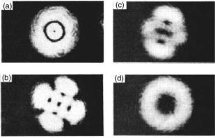
In spite of this insight, the study of optical patterns in nonlinear resonators was abandoned for a decade, and the interest of the optical community turned to spatial e ects in the unidirectional mirrorless propagation of intense light beams in nonlinear materials. In the simplest cases, the spatial evolution of the fields is just a filamentation of the light in a focusing medium; in more complex cases, this evolution leads to the formation of bright spatial solitons [12]. The interest in spatial patterns in lasers was later revived by a series of works. In [13, 14], some nontrivial stationary and dynamic transverse mode formations in laser beams were demonstrated. It was also recognized [15] that the laser Maxwell–Bloch equations admit vortex solutions. The transverse mode formations in [13, 14], and the optical vortices in [15] were related to one another, and the relation was confirmed experimentally (Fig. 1.1) [16, 17]. The optical vortices found in lasers are very similar to the phase defects in speckle fields reported earlier [18, 19].
The above pioneering works were followed by an increasing number of investigations. E orts were devoted to deriving an order parameter equation for lasers and other nonlinear resonators; this would be a simple equation capturing, in the lowest order of approximation, the main spatio-temporal properties of the laser radiation. The Ginzburg–Landau equation, as derived
1.1 Historical Survey |
3 |
Fig. 1.1. The simplest patterns generated by a laser, which can be interpreted as locked transverse modes of a resonator with curved mirrors. From [17], c 1991 American Physical Society
in [11], is just a very simple model equation for lasers with spatial degrees of freedom. Next, attempts were made to derive a more precise order parameter equation for a laser [15, 20], which led to an equation valid for the red detuning limit. Red detuning means that the frequency of the atomic resonance is less than the frequency of the nearest longitudinal mode of the resonator. This equation, however, has a limited validity, since it is not able to predict spontaneous pattern formation: the laser patterns usually appear when the cavity is blue-detuned. Depending on the cavity aperture, higher-order transverse modes [17] or tilted waves [21] can be excited in the blue-detuned resonator.
The problem of the derivation of an order parameter equation for lasers was finally solved in [22, 23], where the complex Swift–Hohenberg (CSH) equation was derived. Compared with the Ginzburg–Landau equation, the CSH equation contains additional nonlocal terms responsible for spatial mode selection, thus inducing a pattern formation instability. Later, the CSH equation for lasers was derived again using a multiscale expansion [24]. The CSH equation describes the spatio-temporal evolution of the field amplitude. Also, an order parameter equation for the laser phase was obtained, in the form of the Kuramoto–Sivashinsky equation [25]. It is noteworthy that both the Swift–Hohenberg and the Kuramoto–Sivashinsky equations appear frequently in the description of hydrodynamic and chemical problems, respectively.
The derivation of an order parameter equation for lasers means a significant advance, since it allows one not only to understand the pattern formation mechanisms in this particular system, but also to consider the broad-aperture laser in the more general context of pattern-forming systems in nature [1].