Doicu A., Wriedt T., Eremin Y.A. Light scattering by systems of particles (OS 124, Springer, 2006

3.3 Homogeneous, Axisymmetric and Nonaxisymmetric Particles

219

DSCS

104					cut sphere - parallel
103
					cut sphere - perpendicular
102					sphere - parallel
					sphere - perpendicular
101
100
10−1
10−2
10−3
10−4	0	30	60	90	120	150	180

Scattering Angle (deg)

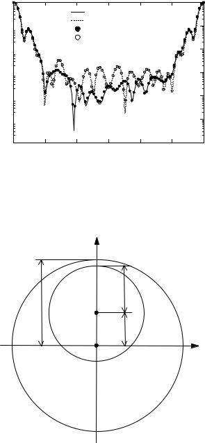
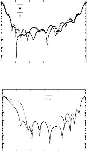
Fig. 3.29. Normalized di erential scattering cross-sections of a sphere and a cut sphere

Fig. 3.30. Geometry of a cube shaped particle with 31,284 faces

with 10132 faces, the Mie parameter computed from the radius is 10, the refractive index is 1.5 and the direction of the incident plane wave is along the z-axis. In Fig. 3.29 the scattering pattern is plotted together with the scattering pattern of a sphere with the same parameters. For better visibility the curves are shifted and it is apparent that there are pronounced di erences in the scattering diagrams of a sphere and a cut sphere.

There are di erent ways to compute scattering by arbitrary particle shapes reconstructed from a number of measured data points. Next we present an example using compactly supported radial basis functions (CS-RBF) for scattered data points processing. For this application we used the software toolkit by Kojekine et al. [121] available from www.karlson.ru. The data points represent a cube shaped particle as depicted in Fig. 3.30 and a number of 378

220 3 Simulation Results

Fig. 3.31. Geometry of a cube shaped particle with 17,680 faces approximated by CS-RBF

	104
	103					cube
						cube cs-rbf
	102
DSCS	101
	100
	10−1
	10−2
	10−3
	10−4	0	30	60	90	120	150	180

Scattering Angle (deg)

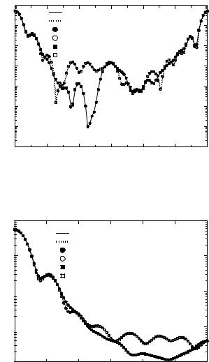
Fig. 3.32. Normalized di erential scattering cross-sections for parallel polarization of a cube and a reconstructed cube

surface points were used in shape reconstruction. The result of the shape reconstruction can be seen in Fig. 3.31, while in Figs. 3.32 and 3.33 the scattering diagrams of the original and the reconstructed cubes are plotted. There are only minor di erences in the backscattering region. The particle shapes have been discretized to a large number of surface patches by using a divide by four scheme and the Rational Reducer Professional software for grid reduction, so that there are finally 17,680 triangular faces with the reconstructed cube.

Scattering results for nonaxisymmetric particles using the superellipsoid as a model particle shape have been given by Wriedt [268]. The program SScaTT (Superellipsoid Scattering Tool) includes a small graphical user interface to generate various superellipsoid particle shape modes and is available

3.4 Inhomogeneous Particles

221

	104
	103					cube
						cube cs-rbf
	102
	101
DSCS	100
10−1
10−2
10−3
10		−4
		0	30	60	90	120	150	180

Scattering Angle (deg)

Fig. 3.33. Normalized di erential scattering cross-sections for perpendicular polarization of a cube and a reconstructed cube

Input Data			Model Control			T matrix of the
			Parameters			inclusion / particles

T-Matrix Routine

T Matrix		Scattering		Convergence Test
		Characteristics		Results

Fig. 3.34. Flow diagram of the TINHOM routine

on CD-ROM with this book. The e ect of particle surface discretization on the computed scattering patterns has been analyzed by Hellmers and Wriedt [99].

3.4 Inhomogeneous Particles

This section discusses numerical and practical aspects of T -matrix calculations for inhomogeneous particles. The flow diagram of the TINHOM routine is shown in Fig. 3.34. The program supports scattering computation for axisymmetric and dielectric host particles with real refractive index. The main feature of this routine is that the T -matrix of the inclusion is provided as input parameter. The inclusion can be a homogeneous, axisymmetric or

222 3 Simulation Results

z

z1 a1

β1

x

O

x1

b1

r

Fig. 3.35. Geometry of an inhomogeneous sphere with a spheroidal inclusion

nonaxisymmetric particle, a composite or a layered scatterer and an aggregate. This choice enables the analysis of particles with complex structure and enhances the flexibility of the program. For computing the T -matrix of the inclusion, the refractive index of the ambient medium must be identical with the relative refractive index of host particle.

We consider an inhomogeneous sphere of radius ksr = 10 as shown in Fig. 3.35. The inhomogeneity is a prolate spheroid of semi-axes ksa1 = 5 and ksb1 = 5. The relative refractive indices of the sphere and the spheroid with respect to the ambient medium are mr = 1.2 and mr1 = 1.5, respectively, and the Euler angles specifying the orientation of the prolate spheroid with respect to the particle coordinate system are αp1 = βp1 = 45◦. The di erential scattering cross-sections are calculated for the case of normal incidence, and the maximum expansion and azimuthal orders for computing the inclusion T matrix are Nrank = 10 and Mrank = 5, respectively. In Fig. 3.36, we compare the T -matrix results to those obtained with the multiple multipole method. The agreement between the scattering curves is acceptable.

In Fig. 3.37, we show an inhomogeneous sphere with a spherical inclusion. The radii of the host sphere and the inclusion are R = 1.0 µm and r = 0.5 µm, respectively, while the relative refractive indices with respect to the ambient medium are mr = 1.33 and mr1 = 1.5, respectively. The inhomogeneity is placed at the distance z1 = 0.25 µm with respect to the particle coordinate system and the wavelength of the incident radiation is chosen as λ = 0.6328 µm.

3.4 Inhomogeneous Particles

223

DSCS

100

10−1

10−2

10−3

10−4

10−5

10−60

TINHOM - parallel

TINHOM - perpendicular

MMP - parallel

MMP - perpendicular

60

120

180

240

300

360

Scattering Angle (deg)

Fig. 3.36. Normalized di erential scattering cross-sections of an inhomogeneous sphere with a spheroidal inclusion. The results are computed with the TINHOM routine and the multiple multipole method (MMP)

z

	r
R
O1
	z1	x
O

Fig. 3.37. Geometry of an inhomogeneous sphere with a spherical inclusion

224 3 Simulation Results

DSCS

2

10				TINHOM2SPH - parallel
1				TINHOM2SPH - perpendicular
10				code of Videen - parallel
0				code of Videen - perpendicular
10
−1
10
−2
10
−3
10
−4
10
−5
10	0	60	120	180	240	300	360

Scattering Angle (deg)

Fig. 3.38. Normalized di erential scattering cross-sections of an inhomogeneous sphere with a spherical inclusion

The results of the di erential scattering cross-sections computed with the TINHOM2SPH routine and the code developed by Videen et al. [243] are shown in Fig. 3.38. The plots demonstrate a complete agreement between the scattering curves. We note that the FORTRAN code developed by Videen et al. [243] (see also, [180]), uses the Lorenz–Mie theory to represent the electromagnetic fields. To exploit the orthogonality of the vector spherical wave functions, the translation addition theorem is used to re-expand the field scattered by the inhomogeneity about the origin of the host sphere.

In order to provide a numerical test of the accuracy of the recursive T - matrix algorithm described in Sect. 2.6, we consider an inhomogeneous sphere with multiple spherical inclusions. The radius of the spherical inclusions is ksr = 0.3, and the maximum expansion and azimuthal orders for computing the inclusion T -matrix are Nrank = Mrank = 3. The radius of the host sphere is ksR = ksRcs(1) = 3.5 and 200 inhomogeneities are generated by using the sequential addition method [47]. The relative refractive indices with respect to the ambient medium are mr = 1.2 and mr1 = 1.5. According to the guidelines of the recursive T -matrix algorithm, two auxiliary surfaces of radii ksRcs(2) = 2.7 and ksRcs(3) = 2.2 are considered in the interior of the host particle. The values of the maximum expansion and azimuthal orders for each auxiliary surface are given in Table 3.5. The matrix inversion is performed with the bi-conjugate gradient method instead of the LU-factorization method. The results presented in Fig. 3.39 correspond to the direct method and the recursive algorithm with one and two auxiliary surfaces. The agreement between the scattering curves is satisfactory, and note that the recursive algorithm with two auxiliary surfaces is faster by a factor of 2 than the direct method.

3.5 Layered Particles

225

Table 3.5. Maximum expansion and azimuthal orders for the auxiliary surfaces

Auxiliary surface	Nrank	Mrank
1	8	5
2	6	4
3	6	4

DSCS

−1

10				parallel - direct method
				parallel - RTA with 1 surface
				parallel - RTA with 2 surfaces
−2				perpendicular - direct method
10				perpendicular - RTA with 1 surface
				perpendicular - RTA with 2 surfaces
−3
10
−4
10
−5
10	0	30	60	90	120	150	180

Scattering Angle (deg)

Fig. 3.39. Normalized di erential scattering cross-sections of an inhomogeneous sphere with multiple spherical inclusions

3.5 Layered Particles

In the following examples we consider electromagnetic scattering by axisymmetric, layered particles. An axisymmetric, layered particle is an inhomogeneous particle consisting of several consecutively enclosing and rotationally symmetric surfaces with a common axis of symmetry. The scattering computations are performed with the TLAY routine and the set of routines devoted to the analysis of inhomogeneous particles. Particle geometries currently supported by the TLAY routine include layered spheroids and cylinders. We note that localized and distributed sources can be used for T -matrix calculations, and in contrast to the TINHOM routine, the relative refractive index of the host particle can be a complex quantity (absorbing dielectric medium).

Figure 3.40 shows a layered spheroid with ksa = 10, ksb = 8, ksa1 = 8, ksb1 = 3 and ksz1 = 3. The relative refractive indices of the host spheroid and the inhomogeneity with respect to the ambient medium are mr = 1.2 and mr1 = 1.5, respectively. Numerical results are presented as plots of the di erential scattering cross-sections for the inhomogeneous spheroid in fixed or random orientation. The scattering characteristics are computed with localized and distributed sources, whereas the distributed sources are placed

226 3 Simulation Results

z

a1 a

O1

z1

O

b1

b

Fig. 3.40. Geometry of a layered spheroid

Table 3.6. Parameters of calculation for an oblate layered spheroid

Type of sources Nrank-host particle		Nrank-inclusion Nint
Localized	17	12	500
Distributed	14	8	2,000

along the symmetry axis of the prolate spheroids. The maximum expansion orders are Nrank = 20 for the host spheroid and Nrank = 13 for the inclusion. The global number of integration points is Nint = 200 for localized sources, and Nint = 1000 for distributed sources. The TINHOM routine uses as input parameter the inclusion T -matrix, which is characterized by Nrank = 13 and Mrank = 5. The results presented in Figs. 3.41 and 3.42 show a complete agreement between the di erent methods.

Scattering by oblate spheroids can be computed with localized and discrete sources distributed in the complex plane. Figure 3.43 compares results obtained with localized and distributed sources for an oblate layered spheroid with ksa = 5, ksb = 10, ksa1 = 3 and ksb1 = 5. The relative refractive indices are mr = 1.2 and mr1 = 1.5, and the parameters of calculation are given in Table 3.6.

						3.5	Layered Particles		227
	101			TLAY - localized sources - parallel
	100			TLAY - localized sources - perpendicular
				TLAY - distributed sources - parallel
	10−1			TLAY - distributed sources - perpendicular
				TINHOM - parallel
				TINHOM - perpendicular
DSCS	10−2
	−3
	10
	10−4
	10−5
	−6
	10	0	60	120	180	240	300	360
				Scattering Angle (deg)

Fig. 3.41. Normalized di erential scattering cross-sections of a layered spheroid

<DSCS>

101
	TLAY - localized sources - parallel
	TLAY - localized sources - perpendicular
100	TLAY - distributed sources - parallel
	TLAY - distributed sources - perpendicular
	TINHOM - parallel
	TINHOM - perpendicular

10−1

10−2

−3
10	0	30	60	90	120	150	180

Scattering Angle (deg)

Fig. 3.42. Averaged di erential scattering cross-sections of a layered spheroid

For highly elongated particles, distributed sources are required to achieve convergence. The results plotted in Fig. 3.44 correspond to a layered cylinder with ksL = 10, ksr = 2, ksL1 = 5 and ksr1 = 1 (Fig. 3.45). The relative refractive indices of the host particle and the inclusions are mr = 1.2 and mr1 = 1.4, respectively. The maximum expansion orders are Nrank = 14 for

228 3 Simulation Results

DSCS

101
100			parallel - distributed sources
			parallel - localized sources
10−1			perpendicular - distributed sources
			perpendicular - localized sources
10−2
10−3
10−4
10−5
10−6
10−7	0	60	120	180	240	300	360
			Scattering Angle (deg)

Fig. 3.43. Normalized di erential scattering cross-sections of an oblate layered spheroid

	100
	10−1				parallel
					perpendicular
	10−2
	10−3
DSCS	10−4
	10−5
	10−6
	10−7
	10−80	60	120	180	240	300	360
			Scattering Angle (deg)

Fig. 3.44. Normalized di erential scattering cross-sections of a layered cylinder

the host particle and Nrank = 8 for the inclusion, while the global number of integration points is Nint = 1,000.

In the next example, the host particle is a sphere of radius ksR = 10, the inclusion is a prolate spheroid with ksa1 = 8 and ksb1 = 3, and the relative refractive indices are mr = 1.2 and mr1 = 1.5. Figures 3.46 and 3.47 compare results obtained with the routines TLAY, TINHOMSPH and TINHOM. The agreement between the scattering curves is very good.