

Hahnel ABCs of Political Economy Modern Primer
.pdf106 The ABCs of Political Economy
THE PRICE OF POWER GAME
When people in an economic relationship have unequal power the logic of preserving a power advantage can lead to a loss of economic efficiency. This dynamic is illustrated by the “Price of Power Game” which helps explain phenomena as diverse as why employers sometimes choose a less efficient technology over a more efficient one, and why patriarchal husbands sometimes bar their wives from working outside the home even when household well being would be increased if the wife did work outside.
Assume P and W combine to produce an economic value and divide the benefit between them. They have been producing a value of 15, but because P has a power advantage in the relationship P has been getting twice as much as W. So initially P and W jointly produce 15, P gets 10 and W gets 5. A new possibility arises that would allow them to produce a greater value. Assume it increases the value of what they jointly produce by 20%, i.e. by 3, raising the value of their combined production from 15 to 18. But taking advantage of the new, more productive possibility also has the effect of increasing W’s power relative to P. Assume the effect of producing the greater value renders W as powerful as P eliminating P’s power advantage. The obvious intuition is that if P stands to lose more from receiving a smaller slice than P stands to gain from having a larger pie to divide with W, it will be in P’s interest to block the efficiency gain. We can call this efficiency loss “the price of power.” But constructing a simple “game tree” helps us understand the obstacles that prevent untying this Gordian knot as well as the logic leading to the unfortunate result.
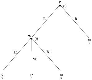
As the player with the power advantage P gets to make the first move at the first “node.” P has two choices at node 1: P can reject the new, more productive possibility and end the game. We call this choice R (for “right” in the game tree diagram in Figure 5.1), and the payoff for P is 10 (listed on top) and the payoff for W is 5 (listed on the bottom) if P chooses R. Or, P can defer to W allowing W to choose whether or not they will adopt the new possibility. We call this choice L (for “left” in the game tree diagram in Figure 5.1), and the payoffs for P and W in this case depend on what W chooses at the second node. If the game gets to the second node because P deferred to W at the first node, W has three choices at node 2: Choice R1 is for W to reject the new possibility and of course the payoffs remain 10 for P and 5 for W as before. Choice L1 is for W to
Micro Economic Models 107
Figure 5.1 Price of Power Game
choose the new, more productive possibility and insist on dividing the larger value of 18 equally between them since the new process empowers W to the extent that P no longer has a power advantage in their relationship, and therefore W can command an equal share with P. If W chooses L1 the payoff for P is therefore 9 and the payoff for W is also 9. Finally, choice M1 (for “middle” in the game tree in Figure 5.1) is for W to choose the new, more productive possibility but to offer to continue to split the pie as before, with P receiving twice as much as W. In other words in M1 W promises P not to take advantage of her new power, which means that P still gets twice as much as W, but since the pie is larger now P’s payoff is 12 and W’s payoff is 6 if W chooses M1 at node 2.
We solve this simple dynamic game by backwards induction. If given the opportunity, W should choose L1 at node 2 since W receives 9 for choice L1 and only 5 for choice R1 and only 6 for choice M1. Knowing that W will choose L1 if the game goes to node 2, P compares a payoff of 10 by choosing R with an expected payoff of 9 if P chooses L and W subsequently chooses L1 as P has every reason to believe she will. Consequently P chooses R at node 1 ending the game and effectively “blocking” the new, more productive possibility.
108 The ABCs of Political Economy
The outcome of the game is not only unequal – P continues to receive twice as much as W – it is also inefficient. One way to see the inefficiency is that while P and W could have produced and shared a total value of 18 they end up only producing and sharing a total value of 15. Another way to see the inefficiency is to note that there is a Pareto superior outcome to (R). (L,M1) is technically possible and has a payoff of 12 for P and 6 for W, compared to the payoff of 10 for P and 5 for W that is the “equilibrium outcome” of the game.
It is the existence of L1 as an option for W at node 2 that forces P to choose R at node 1. Notice that if L1 were eliminated so that W had only two choices at node 2, R1 and M1, W would choose M1 in this new game, in which case P would choose L instead of R at node 1. While this outcome would remain unequal it would not be inefficient. So one could say the inefficiency of the outcome to the original game is because W cannot make a credible promise to P to reject option L1 if the game gets to node 2. Since there is no reason for P to believe W would actually choose M1 over L1 if the game gets to node 2, P chooses R at node 1. In effect P will block an efficiency gain whenever it diminishes P’s power advantage sufficiently. If P stands to lose more from a loss of power than he gains from a bigger pie to divide, P will use his power advantage to block an efficiency gain.
If we turn our attention to how the efficiency loss might be avoided, two possibilities arise. The most straightforward solution, that not only avoids the efficiency loss but generates equal instead of unequal outcomes for P and W, is to eliminate P’s power advantage. If P and W have equal power and divide the value of their joint production equally they will always choose to produce the larger pie and there will never be any efficiency losses. The more convoluted solution is to accept P’s power advantage as a given, and search for ways to make credible a promise from W not to take advantage of her enhanced power. Is there some way to transform the initial game so that a promise from P not to choose L1 is credible?
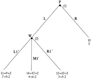
What if W offered P 2 units of “value” to choose L rather than R at node 1? If a contract could be devised in which W had to pay P 2 units, if and only if P chose L at node 1, then the new game would have the following payoffs at node 2: If W chose R1' P would get 10 + 2 =12 instead of 10, and W would get 5 – 2 = 3 instead of 5. If W chose M1' P would get 12 + 2 = 14 instead of 12 and W would get 6
– 2 = 4 instead of 6. Finally, if W chose L1' P would get 9 + 2 = 11 instead of 9 and W would get 9 – 2 = 7 instead of 9. Under these circumstances, in the Transformed Price of Power Game illustrated in
Micro Economic Models 109
Figure 5.2 Transformed Price of Power Game
Figure 5.2 W would choose L1' since 7 is greater than both 4 and 3. But when W chooses L1' at node 2 that gives P 11 which is more than P gets by choosing R at node 1. Therefore a bribe of 2 paid by W to P if and only if P chooses R over L would give us an efficient but unequal outcome. It is efficient because P and W produce 18 instead of 15 and because (L,L1') is Pareto superior to (R). It is still unequal because P receives 11 while W receives only 7.
There are many economic situations where implementing an efficiency gain changes the bargaining power between collaborators and therefore the Price of Power Game can help illustrate aspects of what transpires. Below are two interesting applications.
The price of patriarchy
If P is a patriarchal head of household and W is his wife, the game illustrates one reason why the husband might refuse to permit his wife to work outside the home even though net benefits for the household would be greater if she did.1 Patriarchal power within the household can be modeled as giving the husband the “first mover
1.I do not mean to imply that there are not many other reasons husbands behave in this way. Nor am I suggesting that any of the reasons are morally justifiable, including the reason this model explains.
110 The ABCs of Political Economy
advantage” in our model. Patriarchal power in the economy can be modeled as a gender-based wage gap for women with no labor market experience. If we assume that as long as the wife has not worked outside the home she cannot command as high a wage as her husband in the labor market, her exit option is worse than her husband’s should the marriage dissolve. This unequal exit option makes it possible for a patriarchal husband to insist on a greater share of the household benefits than the wife as long as she has no outside work experience.2 But after she works outside the home for some time the unequal exit option can dissipate, and with it the husband’s power advantage within the home.
The obstacles to eliminating efficiency losses in this situation by eliminating patriarchal advantages are not economic. Gender-based wage discrimination can be eliminated through effective enforcement of laws outlawing discrimination in employment such as those in the US Civil Rights Act. The psychological dynamics that give “first mover” advantages to husbands within marriages requires changes in the attitudes and values of both men and women about gender relations. Of course eliminating the efficiency loss due to patriarchal power by eliminating patriarchal power has the supreme advantage of improving economic justice as well as efficiency.
Trying to eliminate the efficiency loss by making the wife’s promise not to exercise the power advantage she gets by working outside the home credible has a number of disadvantages. Most importantly it is grossly unfair. The bribe the wife must pay her husband to be “allowed” to work outside the home is obviously the result of the disadvantages she suffers from having to negotiate under conditions of unequal and inequitable bargaining power in the first place. Second, it may not be as “practical” as it first appears. Those who believe this solution is more “achievable’ or “practical” than reducing patriarchal privilege should bear in mind how unlikely it is that wives with no labor market credentials could obtain what would amount to an unsecured loan against their future expected productivity gain! Nor could their husbands co-sign for the
2.I am not suggesting that the wife’s lack of work experience in the formal labor market makes her a less productive employee than her husband. If employers do not evaluate the productivity enhancing effects of household work fairly, or use previous employment in the formal sector as a screening device, the effect is the same as if lack of formal sector work experience did, in fact, mean lower productivity. The husband enjoys a power advantage no matter what the reason his wife is paid less than he is initially.
Micro Economic Models 111
loan without effectively changing the payoff numbers in our revised game. Third, even if wives obtained loans from some outside agent
– presumably an institution like the Grameen Bank in Bangladesh that gives loans to women without collateral but holds an entire group of women responsible for non-payment of any of the individual loans – there would have to be a binding legal contract that prevented husbands from taking the bribe and reneging on their promise to allow their wives to work outside the home. Notice that if P can keep the bribe and still choose R he gets 10 + 2 = 12 which is greater than the 11 he gets if he keeps his promise to choose L.
Finally, notice that any bribe between 1 and 4 would successfully transform the game from an inefficient power game to a conceivably efficient, but nonetheless inequitable power game. If W paid P a bribe of 4 the entire efficiency gain would go to her husband. But even if W paid P only a bribe of 1 and kept the entire efficiency gain for herself, she would still end up with less than her husband. In that case W would get 9 – 1 = 8 compared to 9 + 1 = 10 for P. So even if we conjure up a Grameen Bank to give never employed women unsecured loans, even if we ignore all problems and costs of enforcement, there is no way to transform our power game into a game that would deliver equal and equitable outcomes for husbands and wives as well as efficient outcomes. Since P gets 10 by choosing R and ending the game, he must receive at least 10 in order to choose L. But if the productivity gain is only 3 when both work outside, and therefore total household net benefits are only 18, W can receive no more than 8 if P must have at least 10, and no transformation of the game that preserves patriarchal power will produce equitable results. Whether or not this morally inferior solution is actually easier to achieve than reducing patriarchal privilege also seems to be an open question.
Conflict theory of the firm
If P is an employer, or “patron,” and W are his employees or “workers” the Price of Power Game illustrates why an employer might fail to implement a new, more productive technology if that technology is also “employee empowering.” In chapter 10 we consider factors that influence the bargaining power between employers and employees, and therefore the wages employees will receive and the efforts they will have to exert to get them. But one factor that can affect bargaining power in the capitalist firm is the technology used. For example, if an assembly line technology is used
112 The ABCs of Political Economy
and employees are physically separated from one another and unable to communicate during work, it may be more difficult for employees to develop solidarity that would empower them in negotiations with their employer, as compared to a technology that requires workers to work in teams with constant communication between them. Or it may be that one technology requires employees themselves to have a great deal of know-how to carry out their tasks, while another technology concentrates crucial productive knowledge in the hands of a few engineers or supervisors, rendering most employees easily replaceable and therefore less powerful. If the technology that is more productive is also “worker empowering,” employers face the dilemma illustrated by our Price of Power Game and may have reason to choose an inefficient technology over a more efficient one that is less worker empowering.
When we consider possible solutions in this application the situation is somewhat different than in the patriarchal household application. In capitalism there is inevitably a conflict between employers and employees over wages and effort levels. If new technologies not only affect economic efficiency but the relative bargaining power of employers and employees as well, we cannot “trust” the choice of technology to either interested party without running the risk that a more productive technology might be blocked due to detrimental bargaining power effects for whomever has the power to choose. I pointed out above how P might block a more efficient technology if it were sufficiently employee empowering, so we cannot trust employers to choose between technologies. But if W had the power to do so, W might block a more efficient technology if it were sufficiently employer empowering, so we cannot resolve the dilemma by giving unions the say over technology in capitalism either. The solution seems to lie in eliminating the conflict between employers and employees. This can only happen in economies where there are no employers and employees and no division between profits and wages, that is, in economies where employees manage and pay themselves. We consider economies of this kind in chapter 11.
INCOME DISTRIBUTION, PRICES AND TECHNICAL CHANGE
Mainstream economic theory explains the prices of goods and services in terms of consumer preferences, production technologies, and the relative scarcities of different productive resources. Political
Micro Economic Models 113
economists, on the other hand, have long insisted that wages, profits and rents are determined by power relations among classes in addition to factors mainstream economic theory takes into account, and therefore that the relative prices of goods in capitalist economies depend on power relations between classes as well as on consumer preferences and production technologies.
The labor theory of value Karl Marx developed in Das Kapital was the first political economy explanation of “wage, price and profit”3 determination. In Production of Commodities by Means of Commodities (Cambridge University Press, 1960) Piero Sraffa presented an alternative political economy explanation that avoided logical inconsistencies and anomalies in the labor theory of value, and extends easily to include different wage rates for different kinds of labor and rents on different kinds of natural resources – which the labor theory of value could not. The model below is based on Sraffa’s theory, and is often called “the modern surplus approach.”4
3.Karl Marx wrote a pamphlet under this title in which he presented a popularized version of the labor theory of value from Das Kapital.
4.The “surplus approach” is only one part of a political economy explanation of the determination of wages, profits, rents, and prices. The surplus approach does not explain why consumers come to have the preferences they do, nor what determines the relative power of employers, workers, and resource owners. Instead the surplus approach takes consumer demand and the power relationships between workers, employers, and resource owners as givens, and seeks to explain what prices will result under those conditions. While it does not explain what causes changes in the power relations between workers, employers, and resource owners, the surplus approach does explain how any changes in power between them will affect prices as well as income distribution. And while it does not explain what causes technological innovations, it does explain which new technologies will be chosen, and how their implementation will affect wages, profits, rents, prices, and economic efficiency. Logically, the surplus approach is the last part of a micro political economy. Other political economy theories must explain the factors that influence preference formation and power relations between different classes. In chapter 4 the effect of market bias on preference formation was treated briefly. In chapter 10 factors affecting the bargaining power of workers and capitalists are explored. For a more rigorous political economy theory of “endogenous preferences” see chapter 6 in Hahnel and Albert, Quiet Revolution in Welfare Economics. See chapters 2 and 8 for a more thorough presentation and defense of the “conflict theory of the firm” and a more thorough examination of the factors that influence the bargaining power of capitalists and workers. But once consumer demand and the bargaining power between classes is given, the “surplus approach,” or Sraffa model, provides a rigorous explanation of price formation and income distribution in capitalism.
114 The ABCs of Political Economy
The Sraffa model
Assume a two sector economy defined by the technology below where a(ij) is the number of units of good i needed to produce 1 unit of good j, and L(j) is the number of hours of labor needed to produce 1 unit of good j. Suppose:
a(11) = 0.3 |
a(12) = 0.2 |
a(21) = 0.2 |
a(22) = 0.4 |
L(1) = 0.1 |
L(2) = 0.2 |
The first column can be read as a “recipe” for making 1 unit of good
1:It takes 0.3 units of good 1 itself, 0.2 units of good 2, and 0.1 hour of labor to “stir” these ingredients to get 1 unit of good 1 as output. Similarly, the second column is a recipe for making 1 unit of good
2:It takes 0.2 units of good 1, 0.4 units of good 2 itself, and 0.2 hours of labor to make 1 unit of good 2.
Let p(i) be the price of a unit of good i, w be the hourly wage rate, and r(i) be the rate of profit received by capitalists in sector i. The first step is to write down an equation for each industry that expresses the truism that revenue minus cost for the industry is, by definition, equal to industry profit. If we divide both sides of this equation by the number of units of output the industry produces we get the truism that revenue per unit of output minus cost per unit of output must equal profit per unit of output. Another way of saying this is: cost per unit of output plus profit per unit of output must equal revenue per unit of output. This is the equation we want to write for each industry.
The second step is to write down what cost per unit of output and revenue per unit of output will be for each industry. For industry 1 it takes a(11) units of good 1 itself to make a unit of output of good 1. That will cost p(1)a(11). It also takes a(21) units of good 2 to make a unit of output of good 1. That will cost p(2)a(21). So [p(1)a(11) + p(2)a(21)] are the non-labor costs of making 1 unit of good 1. Since it takes L(1) hours of labor to make a unit of good 1 and the wage per hour is w, the labor cost of making a unit of good 1 is wL(1). Revenue per unit of output of good 1 is simply p(1).
What is profit per unit of output in industry 1? By definition profits are revenues minus costs, so profits per unit of output must be equal to revenues per unit of output minus cost per unit of output. Also by definition the rate of profit is profits divided by
Micro Economic Models 115
whatever part of costs a capitalist must pay for in advance. Dividing both the numerator and denominator by the number of units of output in industry 1 gives us the truism that the rate of profit in industry 1 is equal to the profit per unit of output in industry 1 divided by whatever part of costs per unit of output capitalists must advance in industry 1. Therefore, the profit per unit of output in industry 1 must be equal to the rate of profit for industry 1 times the cost per unit of output capitalists must advance in industry 1.
We will assume (with Sraffa) that capitalists must pay for nonlabor costs in advance but can pay their employees after the production period is over out of revenues from the sale of the goods produced. So the cost per unit of output capitalists must advance in industry 1 is only the non-labor costs per unit, or [p(1)a(11) + p(2)a(21)]. We will also assume (with Sraffa) that the rate of profit capitalists receive is the same in both industries, r.5 Therefore:
profit per unit of output in industry 1 = r[p(1)a(11) + p(2)a(21)]
And we are ready to write the accounting identity, or truism, that cost per unit of output plus profit per unit of output equals revenue per unit of output in industry 1:
[p(1)a(11) + p(2)a(21)] + wL(1) + r[p(1)a(11) + p(2)a(21)] = p(1)
Which can be rewritten for convenience as:
(1)(1+r) [p(1)a(11) + p(2)a(21)] + wL(1) = p(1)
Similarly for industry 2:
(2)(1+r) [p(1)a(12) + p(2)a(22)] + wL(2) = p(2)
5.These assumptions are both convenient because they simplify the analysis. However, they are not necessary, and one of the strengths of the surplus approach is we could change them and still solve the model. In particular, if capitalists in different industries had different bargaining power, or if some industries were more competitive and others less so, or if there were barriers to entry in some industries so capitalists were not free to flee low profit industries and enter high profit ones until profit rates were equal everywhere, we could easily complicate our model and stipulate different rates of profit r(1) and r(2) for the two industries.