TsOS / DSP_guide_Smith / Ch17

CHAPTER

Custom Filters

17

Most filters have one of the four standard frequency responses: low-pass, high-pass, band-pass or band-reject. This chapter presents a general method of designing digital filters with an arbitrary frequency response, tailored to the needs of your particular application. DSP excels in this area, solving problems that are far above the capabilities of analog electronics. Two important uses of custom filters are discussed in this chapter: deconvolution, a way of restoring signals that have undergone an unwanted convolution, and optimal filtering, the problem of separating signals with overlapping frequency spectra. This is DSP at its best.

Arbitrary Frequency Response

The approach used to derive the windowed-sinc filter in the last chapter can also be used to design filters with virtually any frequency response. The only difference is how the desired response is moved from the frequency domain into the time domain. In the windowed-sinc filter, the frequency response and the filter kernel are both represented by equations, and the conversion between them is made by evaluating the mathematics of the Fourier transform. In the method presented here, both signals are represented by arrays of numbers, with a computer program (the FFT) being used to find one from the other.

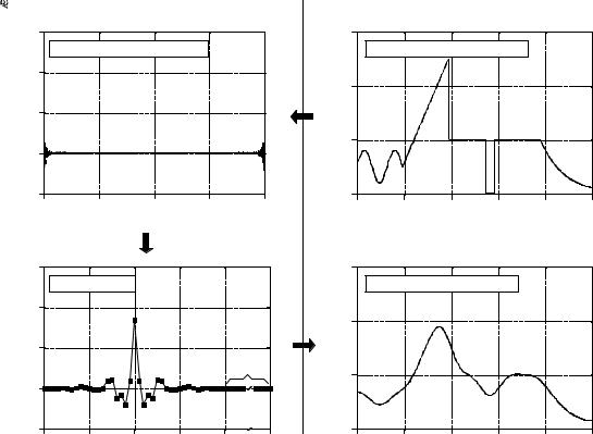
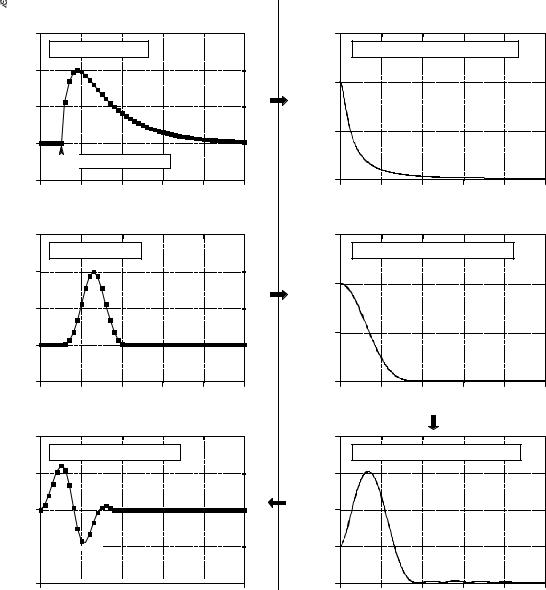
Figure 17-1 shows an example of how this works. The frequency response we want the filter to produce is shown in (a). To say the least, it is very irregular and would be virtually impossible to obtain with analog electronics. This ideal frequency response is defined by an array of numbers that have been selected, not some mathematical equation. In this example, there are 513 samples spread between 0 and 0.5 of the sampling rate. More points could be used to better represent the desired frequency response, while a smaller number may be needed to reduce the computation time during the filter design. However, these concerns are usually small, and 513 is a good length for most applications.

297

298	The Scientist and Engineer's Guide to Digital Signal Processing

Besides the desired m a g n i t u d e array shown in (a), there must be a corresponding phase array of the same length. In this example, the phase of the desired frequency response is entirely zero (this array is not shown in Fig. 17-1). Just as with the magnitude array, the phase array can be loaded with any arbitrary curve you would like the filter to produce. However, remember that the first and last samples (i.e., 0 and 512) of the phase array must have a value of zero (or a multiple of 2B, which is the same thing). The frequency response can also be specified in rectangular form by defining the array entries for the real and imaginary parts, instead of using the magnitude and phase.

The next step is to take the Inverse DFT to move the filter into the time domain. The quickest way to do this is to convert the frequency domain to rectangular form, and then use the Inverse FFT. This results in a 1024 sample signal running from 0 to 1023, as shown in (b). This is the impulse response that corresponds to the frequency response we want; however, it is not suitable for use as a filter kernel (more about this shortly). Just as in the last chapter, it needs to be shifted, truncated, and windowed. In this example, we will design the filter kernel with M ' 40 , i.e., 41 points running from sample 0 to sample 40. Table 17-1 shows a computer program that converts the signal in (b) into the filter kernel shown in (c). As with the windowed-sinc filter, the points near the ends of the filter kernel are so small that they appear to be zero when plotted. Don't make the mistake of thinking they can be deleted!

100	'CUSTOM FILTER DESIGN
110	'This program converts an aliased 1024 point impulse response into an M+1 point
120	'filter kernel (such as Fig. 17-1b being converted into Fig. 17-1c)
130	'
140	DIM REX[1023]	'REX[ ] holds the signal being converted
150	DIM T[1023]	'T[ ] is a temporary storage buffer
160	'
170	PI = 3.14159265
180	M% = 40	'Set filter kernel length (41 total points)
190	'
200	GOSUB XXXX	'Mythical subroutine to load REX[ ] with impulse response
210	'
220	FOR I% = 0 TO 1023 'Shift (rotate) the signal M/2 points to the right
230	INDEX% = I% + M%/2
240	IF INDEX% > 1023 THEN INDEX% = INDEX%-1024
250	T[INDEX%] = REX[I%]
260 NEXT I%
270	'
280 FOR I% = 0 TO 1023
290	REX[I%] = T[I%]
300 NEXT I%
310	'	'Truncate and window the signal
320 FOR I% = 0 TO 1023
330	IF I% <= M% THEN REX[I%] = REX[I%] * (0.54 - 0.46 * COS(2*PI*I%/M%))
340	IF I% > M% THEN REX[I%] = 0
350 NEXT I%
360	'	'The filter kernel now resides in REX[0] to REX[40]
370 END		TABLE 17-1

Chapter 17Custom Filters

299

Time Domain

	1.5
		b. Impulse response (aliased)
Amplitude	1.0
	0.5
	0.0
	-0.5
	0	256	512	768	10234

Sample number

	1.5
		c. Filter kernel
	1.0
Amplitude	0.5
						added
						zeros
	0.0
	-0.5
	0	10	20	30	40	102350

Sample number

Frequency Domain

	3
		a. Desired frequency response
Amplitude	2
	1
	0
	0	0.1	0.2	0.3	0.4	0.5
			Frequency
	3

d. Actual frequency response

Amplitude	2
	1
	0
	0	0.1	0.2	0.3	0.4	0.5

Frequency

FIGURE 17-1

Example of FIR filter design. Figure (a) shows the desired frequency response, with 513 samples running between 0 to 0.5 of the sampling rate. Taking the Inverse DFT results in (b), an aliased impulse response composed of 1024 samples. To form the filter kernel, (c), the aliased impulse response is truncated to M% 1 samples, shifted to the right by M/2 samples, and multiplied by a Hamming or Blackman window. In this example, M is 40. The program in Table 17-1 shows how this is done. The filter kernel is tested by padding it with zeros and taking the DFT, providing the actual frequency response of the filter, (d).

The last step is to test the filter kernel. This is done by taking the DFT (using the FFT) to find the actual frequency response, as shown in (d). To obtain better resolution in the frequency domain, pad the filter kernel with zeros before the FFT. For instance, using 1024 total samples (41 in the filter kernel, plus 983 zeros), results in 513 samples between 0 and 0.5.

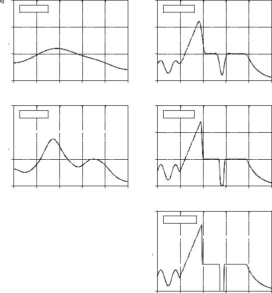
As shown in Fig. 17-2, the length of the filter kernel determines how well the actual frequency response matches the desired frequency response. The exceptional performance of FIR digital filters is apparent; virtually any frequency response can be obtained if a long enough filter kernel is used.

This is the entire design method; however, there is a subtle theoretical issue that needs to be clarified. Why isn't it possible to directly use the impulse response shown in 17-1b as the filter kernel? After all, if (a) is the Fourier transform of (b), wouldn't convolving an input signal with (b) produce the exact frequency response we want? The answer is no, and here's why.

300	The Scientist and Engineer's Guide to Digital Signal Processing

When designing a custom filter, the desired frequency response is defined by the values in an array. Now consider this: what does the frequency response do between the specified points? For simplicity, two cases can be imagined, one "good" and one "bad." In the "good" case, the frequency response is a smooth curve between the defined samples. In the "bad" case, there are wild fluctuations between. As luck would have it, the impulse response in (b) corresponds to the "bad" frequency response. This can be shown by padding it with a large number of zeros, and then taking the DFT. The frequency response obtained by this method will show the erratic behavior between the originally defined samples, and look just awful.

To understand this, imagine that we force the frequency response to be what we want by defining it at an infinite number of points between 0 and 0.5. That is, we create a continuous curve. The inverse DTFT is then used to find the impulse response, which will be infinite in length. In other words, the "good" frequency response corresponds to something that cannot be represented in a computer, an infinitely long impulse response. When we represent the frequency spectrum with N/2 % 1 samples, only N points are provided in the time domain, making it unable to correctly contain the signal. The result is that the infinitely long impulse response wraps up (aliases) into the N points. When this aliasing occurs, the frequency response changes from "good" to "bad." Fortunately, windowing the N point impulse response greatly reduces this aliasing, providing a smooth curve between the frequency domain samples.

Designing a digital filter to produce a given frequency response is quite simple. The hard part is finding what frequency response to use. Let's look at some strategies used in DSP to design custom filters.

Deconvolution

Unwanted convolution is an inherent problem in transferring analog information. For instance, all of the following can be modeled as a convolution: image blurring in a shaky camera, echoes in long distance telephone calls, the finite bandwidth of analog sensors and electronics, etc. Deconvolution is the process of filtering a signal to compensate for an undesired convolution. The goal of deconvolution is to recreate the signal as it existed before the convolution took place. This usually requires the characteristics of the convolution (i.e., the impulse or frequency response) to be known. This can be distinguished from blind deconvolution, where the characteristics of the parasitic convolution are not known. Blind deconvolution is a much more difficult problem that has no general solution, and the approach must be tailored to the particular application.

Deconvolution is nearly impossible to understand in the time domain, but quite straightforward in the frequency domain. Each sinusoid that composes the original signal can be changed in amplitude and/or phase as it passes through the undesired convolution. To extract the original signal, the deconvolution filter must undo these amplitude and phase changes. For

Chapter 17Custom Filters

301

3
	a. M = 10
2
Amplitude
1
0
0	0.1	0.2	0.3	0.4	0.5
		Frequency
3
	b. M = 30

2

Amplitude

1

0

0

0.1

0.2

0.3

0.4

0.5

Frequency

FIGURE 17-2

Frequency response vs. filter kernel length. These figures show the frequency responses obtained with various lengths of filter kernels. The number of points in each filter kernel is equal to M% 1 , running from 0 to M. As more points are used in the filter kernel, the resulting frequency response more closely matches the desired frequency response. Figure 17-1a shows the desired frequency response for this example.

3
	c. M = 100
2
Amplitude
1
0
0	0.1	0.2	0.3	0.4	0.5
		Frequency
3
	d. M = 300
2
Amplitude
1
0
0	0.1	0.2	0.3	0.4	0.5
		Frequency
3
	e. M = 1000

2

Amplitude

1

0

0

0.1

0.2

0.3

0.4

0.5

Frequency

example, if the convolution changes a sinusoid's amplitude by 0.5 with a 30 degree phase shift, the deconvolution filter must amplify the sinusoid by 2.0 with a -30 degree phase change.

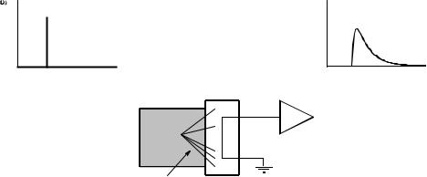
The example we will use to illustrate deconvolution is a gamma ray detector. As illustrated in Fig. 17-3, this device is composed of two parts, a scintillator and a light detector. A scintillator is a special type of transparent material, such as sodium iodide or bismuth germanate. These compounds change the energy in each gamma ray into a brief burst of visible light. This light

302	The Scientist and Engineer's Guide to Digital Signal Processing

Energy

Voltage

Time

Time

scintillator

gamma ray amplifier

light	light detector

FIGURE 17-3

Example of an unavoidable convolution. A gamma ray detector can be formed by mounting a scintillator on a light detector. When a gamma ray strikes the scintillator, its energy is converted into a pulse of light. This pulse of light is then converted into an electronic signal by the light detector. The gamma ray is an impulse, while the output of the detector (i.e., the impulse response) resembles a one-sided exponential.

is then converted into an electronic signal by a light detector, such as a photodiode or photomultiplier tube. Each pulse produced by the detector resembles a one-sided exponential, with some rounding of the corners. This shape is determined by the characteristics of the scintillator used. When a gamma ray deposits its energy into the scintillator, nearby atoms are excited to a higher energy level. These atoms randomly deexcite, each producing a single photon of visible light. The net result is a light pulse whose amplitude decays over a few hundred nanoseconds (for sodium iodide). Since the arrival of each gamma ray is an impulse, the output pulse from the detector (i.e., the one-sided exponential) is the impulse response of the system.

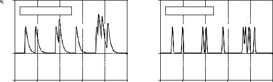
Figure 17-4a shows pulses generated by the detector in response to randomly arriving gamma rays. The information we would like to extract from this output signal is the amplitude of each pulse, which is proportional to the energy of the gamma ray that generated it. This is useful information because the energy can tell interesting things about where the gamma ray has been. For example, it may provide medical information on a patient, tell the age of a distant galaxy, detect a bomb in airline luggage, etc.

Everything would be fine if only an occasional gamma ray were detected, but this is usually not the case. As shown in (a), two or more pulses may overlap, shifting the measured amplitude. One answer to this problem is to deconvolve the detector's output signal, making the pulses narrower so that less pile-up occurs. Ideally, we would like each pulse to resemble the original impulse. As you may suspect, this isn't possible and we must settle for a pulse that is finite in length, but significantly shorter than the detected pulse. This goal is illustrated in Fig. 17-4b.

Chapter 17Custom Filters

303

2

a. Detected pulses

1

Amplitude
0
-1
0	100	200	300	400	500

Sample number

2

b. Filtered pulses

1

Amplitude
0
-1
0	100	200	300	400	500

Sample number

FIGURE 17-4

Example of deconvolution. Figure (a) shows the output signal from a gamma ray detector in response to a series of randomly arriving gamma rays. The deconvolution filter is designed to convert (a) into (b), by reducing the width of the pulses. This minimizes the amplitude shift when pulses land on top of each other.

Even though the detector signal has its information encoded in the time domain, much of our analysis must be done in the frequency domain, where the problem is easier to understand. Figure 17-5a is the signal produced by the detector (something we know). Figure (c) is the signal we wish to have (also something we know). This desired pulse was arbitrarily selected to be the same shape as a Blackman window, with a length about one-third that of the original pulse. Our goal is to find a filter kernel, (e), that when convolved with the signal in (a), produces the signal in (c). In equation form: if a te ' c , and given a and c, find e.

If these signals were combined by addition or multiplication instead of convolution, the solution would be easy: subtraction is used to "de-add" and division is used to "de-multiply." Convolution is different; there is not a simple inverse operation that can be called "deconvolution." Convolution is too messy to be undone by directly manipulating the time domain signals.

Fortunately, this problem is simpler in the frequency domain. Remember, convolution in one domain corresponds with multiplication in the other domain. Again referring to the signals in Fig. 17-5: if b × f ' d , and given b and d, find f. This is an easy problem to solve: the frequency response of the filter, (f), is the frequency spectrum of the desired pulse, (d), divided by the frequency spectrum of the detected pulse, (b). Since the detected pulse is asymmetrical, it will have a nonzero phase. This means that a complex division must be used (that is, a magnitude & phase divided by another magnitude & phase). In case you have forgotten, Chapter 9 defines how to perform a complex division of one spectrum by another. The required filter kernel, (e), is then found from the frequency response by the custom filter method (IDFT, shift, truncate, & multiply by a window).

There are limits to the improvement that deconvolution can provide. In other words, if you get greedy, things will fall apart. Getting greedy in this

304	The Scientist and Engineer's Guide to Digital Signal Processing

example means trying to make the desired pulse excessively narrow. Let's look at what happens. If the desired pulse is made narrower, its frequency spectrum must contain more high frequency components. Since these high frequency components are at a very low amplitude in the detected pulse, the filter must have a very high gain at these frequencies. For instance, (f) shows that some frequencies must be multiplied by a factor of three to achieve the desired pulse in (c). If the desired pulse is made narrower, the gain of the deconvolution filter will be even greater at high frequencies.

The problem is, small errors are very unforgiving in this situation. For instance, if some frequency is amplified by 30, when only 28 is required, the deconvolved signal will probably be a mess. When the deconvolution is pushed to greater levels of performance, the characteristics of the unwanted convolution must be understood with greater accuracy and precision. There are always unknowns in real world applications, caused by such villains as: electronic noise, temperature drift, variation between devices, etc. These unknowns set a limit on how well deconvolution will work.

Even if the unwanted convolution is perfectly understood, there is still a factor that limits the performance of deconvolution: noise. For instance, most unwanted convolutions take the form of a low-pass filter, reducing the amplitude of the high frequency components in the signal. Deconvolution corrects this by amplifying these frequencies. However, if the amplitude of these components falls below the inherent noise of the system, the information contained in these frequencies is lost. No amount of signal processing can retrieve it. It's gone forever. Adios! Goodbye! Sayonara! Trying to reclaim this data will only amplify the noise. As an extreme case, the amplitude of some frequencies may be completely reduced to zero. This not only obliterates the information, it will try to make the deconvolution filter have infinite gain at these frequencies. The solution: design a less aggressive deconvolution filter and/or place limits on how much gain is allowed at any of the frequencies.

How far can you go? How greedy is too greedy? This depends totally on the problem you are attacking. If the signal is well behaved and has low noise, a significant improvement can probably be made (think a factor of 5-10). If the signal changes over time, isn't especially well understood, or is noisy, you won't do nearly as well (think a factor of 1-2). Successful deconvolution involves a great deal of testing. If it works at some level, try going farther; you will know when it falls apart. No amount of theoretical work will allow you to bypass this iterative process.

Deconvolution can also be applied to frequency domain encoded signals. A classic example is the restoration of old recordings of the famous opera singer, Enrico Caruso (1873-1921). These recordings were made with very primitive equipment by modern standards. The most significant problem is the resonances of the long tubular recording horn used to gather the sound. Whenever the singer happens to hit one of these resonance frequencies, the loudness of the recording abruptly increases. Digital deconvolution has improved the subjective quality of these recordings by

Chapter 17Custom Filters

305

Time Domain

1.5

a. Detected pulse

	1.0
Amplitude	0.5
	0.0

Gamma ray strikes

-0.5

0

10

20

30

40

50

Sample number

	1.5
		c. Desired pulse
Amplitude	1.0
	0.5
	0.0
	-0.5
	0	10	20	30	40	50
			Sample number
	0.4
		e. Required filter kernel
Amplitude	0.2
	0.0

-0.2

-0.4 0 10 20 30 40 50

Sample number

		Frequency Domain
	1.5
		b. Detected frequency spectrum
Amplitude	1.0
	0.5
	0.0
	0	0.1	0.2	0.3	0.4	0.5
			Frequency
	1.5
		d. Desired frequency spectrum

Amplitude	1.0
	0.5
	0.0
	0	0.1	0.2	0.3	0.4	0.5
			Frequency
	4.0
		f. Required Frequency response
	3.0
Amplitude	2.0
	1.0
	0.0
	0	0.1	0.2	0.3	0.4	0.5
			Frequency

FIGURE 17-5

Example of deconvolution in the time and frequency domains. The impulse response of the example gamma ray detector is shown in (a), while the desired impulse response is shown in (c). The frequency spectra of these two signals are shown in (b) and (d), respectively. The filter that changes (a) into (c) has a frequency response, (f), equal to (b) divided by (d). The filter kernel of this filter, (e), is then found from the frequency response using the custom filter design method (inverse DFT, truncation, windowing). Only the magnitudes of the frequency domain signals are shown in this illustration; however, the phases are nonzero and must also be used.

reducing the loud spots in the music. We will only describe the general method; for a detailed description, see the original paper: T. Stockham, T. Cannon, and R. Ingebretsen, "Blind Deconvolution Through Digital Signal Processing", Proc. IEEE, vol. 63, Apr. 1975, pp. 678-692.

306	The Scientist and Engineer's Guide to Digital Signal Processing
	a. Original spectrum	c. Recorded spectrum	e. Deconvolved spectrum
	Amplitude	Amplitude	Amplitude
	Frequency	Frequency	Frequency

	Undesired	Deconvolution
	Convolution

b. Frequency response

Amplitude

Frequency

d. Frequency response

Amplitude

Frequency

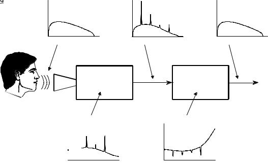
FIGURE 17-6

Deconvolution of old phonograph recordings. The frequency spectrum produced by the original singer is illustrated in (a). Resonance peaks in the primitive equipment, (b), produce distortion in the recorded frequency spectrum, (c). The frequency response of the deconvolution filter, (d), is designed to counteracts the undesired convolution, restoring the original spectrum, (e). These graphs are for illustrative purposes only; they are not actual signals.

Figure 17-6 shows the general approach. The frequency spectrum of the original audio signal is illustrated in (a). Figure (b) shows the frequency response of the recording equipment, a relatively smooth curve except for several sharp resonance peaks. The spectrum of the recorded signal, shown in (c), is equal to the true spectrum, (a), multiplied by the uneven frequency response, (b). The goal of the deconvolution is to counteract the undesired convolution. In other words, the frequency response of the deconvolution filter, (d), must be the inverse of (b). That is, each peak in (b) is cancelled by a corresponding dip in (d). If this filter were perfectly designed, the resulting signal would have a spectrum, (e), identical to that of the original. Here's the catch: the original recording equipment has long been discarded, and its frequency response, (b), is a mystery. In other words, this is a blind deconvolution problem; given only (c), how can we determine (d)?

Blind deconvolution problems are usually attacked by making an estimate or assumption about the unknown parameters. To deal with this example, the average spectrum of the original music is assumed to match the average spectrum of the same music performed by a present day singer using modern equipment. The average spectrum is found by the techniques of Chapter 9: