TsOS / DSP_guide_Smith / Ch19

CHAPTER

Recursive Filters

19

Recursive filters are an efficient way of achieving a long impulse response, without having to perform a long convolution. They execute very rapidly, but have less performance and flexibility than other digital filters. Recursive filters are also called Infinite Impulse Response (IIR) filters, since their impulse responses are composed of decaying exponentials. This distinguishes them from digital filters carried out by convolution, called Finite Impulse Response (FIR) filters. This chapter is an introduction to how recursive filters operate, and how simple members of the family can be designed. Chapters 20, 26 and 33 present more sophisticated design methods.

The Recursive Method

To start the discussion of recursive filters, imagine that you need to extract information from some signal, x[ ]. Your need is so great that you hire an old mathematics professor to process the data for you. The professor's task is to filter x[ ] to produce y[ ], which hopefully contains the information you are interested in. The professor begins his work of calculating each point in y[ ] according to some algorithm that is locked tightly in his over-developed brain. Part way through the task, a most unfortunate event occurs. The professor begins to babble about analytic singularities and fractional transforms, and other demons from a mathematician's nightmare. It is clear that the professor has lost his mind. You watch with anxiety as the professor, and your algorithm, are taken away by several men in white coats.

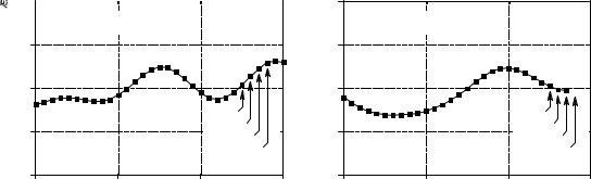
You frantically review the professor's notes to find the algorithm he was using. You find that he had completed the calculation of points y[0] through y[27] , and was about to start on point y[28] . As shown in Fig. 19-1, we will let the variable, n, represent the point that is currently being calculated. This means that y[n] is sample 28 in the output signal, y[n& 1] is sample 27, y[n& 2] is sample 26, etc. Likewise, x[n] is point 28 in the input signal,

319

320	The Scientist and Engineer's Guide to Digital Signal Processing

x[n& 1] is point 27, etc. To understand the algorithm being used, we ask ourselves: "What information was available to the professor to calculate y[n] , the sample currently being worked on?"

The most obvious source of information is the input signal, that is, the values: x[n], x[n& 1], x[n& 2], þ. The professor could have been multiplying each point in the input signal by a coefficient, and adding the products together:

y [n ] ' a0 x [n ] % a1 x [n & 1] % a2 x [n & 2] % a3 x [n & 3] % þ

You should recognize that this is nothing more than simple convolution, with the coefficients: a0, a1, a2, þ, forming the convolution kernel. If this was all the professor was doing, there wouldn't be much need for this story, or this chapter. However, there is another source of information that the professor had access to: the p r e v i o u s l y calculated values of the output signal, held in: y[n& 1], y[n& 2], y[n& 3], þ. Using this additional information, the algorithm would be in the form:

y [n ] ' a0 x [n ] % a1 x [n & 1] % a2 x [n & 2] % a3 x [n & 3] %

% b1 y [n & 1] % b2 y [n & 2] % b3 y [n & 3] %

EQUATION 19-1

The recursion equation. In this equation, x[ ] is the input signal, y[ ] is the output signal, and the a's and b's are coefficients.

þ

þ

In words, each point in the output signal is found by multiplying the values from the input signal by the "a" coefficients, multiplying the previously calculated values from the output signal by the "b" coefficients, and adding the products together. Notice that there isn't a value for b0 , because this corresponds to the sample being calculated. Equation 19-1 is called the recursion equation, and filters that use it are called recursive filters. The "a" and "b" values that define the filter are called the recursion coefficients. In actual practice, no more than about a dozen recursion coefficients can be used or the filter becomes unstable (i.e., the output continually increases or oscillates). Table 19-1 shows an example recursive filter program.

Recursive filters are useful because they bypass a longer convolution. For instance, consider what happens when a delta function is passed through a recursive filter. The output is the filter's impulse response, and will typically be a sinusoidal oscillation that exponentially decays. Since this impulse response in infinitely long, recursive filters are often called infinite impulse response (IIR) filters. In effect, recursive filters convolve the input signal with a very long filter kernel, although only a few coefficients are involved.

Chapter 19Recursive Filters

321

2				2
		a. The input signal, x[ ]			b. The output signal, y[ ]

Amplitude	1				Amplitude	1
	0					0
				x[n-3]
	-1			x[n-2]		-1
				x[n-1]
				x[n]
	-2					-2
	0	10	20	30		0	10	20
		Sample number					Sample number

y[n-3] y[n-2]

y[n-1] y[n]

30

FIGURE 19-1

Recursive filter notation. The output sample being calculated, y[n] , is determined by the values from the input signal, x[n], x[n& 1], x[n& 2], þ, as well as the previously calculated values in the output signal, y[n& 1], y[n& 2], y[n& 3], þ. These figures are shown for n ' 28 .

The relationship between the recursion coefficients and the filter's response is given by a mathematical technique called the z-transform, the topic of Chapter 33. For example, the z-transform can be used for such tasks as: converting between the recursion coefficients and the frequency response, combining cascaded and parallel stages into a single filter, designing recursive systems that mimic analog filters, etc. Unfortunately, the z-transform is very mathematical, and more complicated than most DSP users are willing to deal with. This is the realm of those that specialize in DSP.

There are three ways to find the recursion coefficients without having to understand the z-transform. First, this chapter provides design equations for several types of simple recursive filters. Second, Chapter 20 provides a "cookbook" computer program for designing the more sophisticated Chebyshev low-pass and high-pass filters. Third, Chapter 26 describes an iterative method for designing recursive filters with an arbitrary frequency response.

100	'RECURSIVE FILTER
110	'
120	DIM X[499]	'holds the input signal
130	DIM Y[499]	'holds the filtered output signal
140	'
150	GOSUB XXXX	'mythical subroutine to calculate the recursion
160	'	'coefficients: A0, A1, A2, B1, B2
170	'
180	GOSUB XXXX	'mythical subroutine to load X[ ] with the input data
190	'
200 FOR I% = 2 TO 499
210	Y[I%] = A0*X[I%] + A1*X[I%-1] + A2*X[I%-2] + B1*Y[I%-1] + B2*Y[I%-2]
220 NEXT I%
230	'
240 END		TABLE 19-1

322	The Scientist and Engineer's Guide to Digital Signal Processing

Digital Filter

1.5

1.0

Amplitude	0.5
	0.0
	-0.5
	0	10	20	30	40

Sample number

Recursive

Filter

a0 = 0.15 b1 = 0.85

		1.5
	Amplitude	1.0
		0.5

0.0

-0.5

0

10

20

30

40

Sample number

Analog Filter

1.5

R

1.0

Amplitude	0.5
	0.0
	-0.5
	0	10	20	30

Time

C

	1.5
Amplitude	1.0
	0.5
	0.0
	-0.5
	0	10	20	30	40
			Time

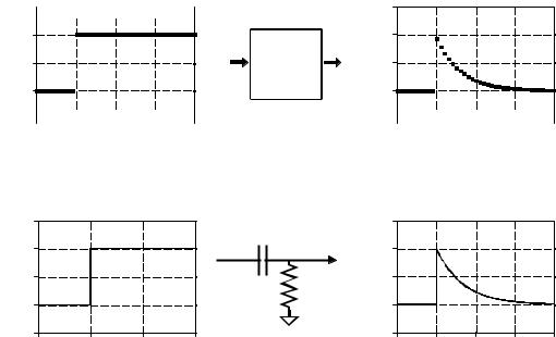
FIGURE 19-2

Single pole low-pass filter. Digital recursive filters can mimic analog filters composed of resistors and capacitors. As shown in this example, a single pole low-pass recursive filter smoothes the edge of a step input, just as an electronic RC filter.

Single Pole Recursive Filters

Figure 19-2 shows an example of what is called a single pole low-pass filter. This recursive filter uses just two coefficients, a0 ' 0.15 and b1 ' 0.85 . For this example, the input signal is a step function. As you should expect for a low-pass filter, the output is a smooth rise to the steady state level. This figure also shows something that ties into your knowledge of electronics. This lowpass recursive filter is completely analogous to an electronic low-pass filter composed of a single resistor and capacitor.

The beauty of the recursive method is in its ability to create a wide variety of responses by changing only a few parameters. For example, Fig. 19-3 shows a filter with three coefficients: a0 ' 0.93 , a1 ' & 0.93 and b1 ' 0.86 . As shown by the similar step responses, this digital filter mimics an electronic RC high-pass filter.

These single pole recursive filters are definitely something you want to keep in your DSP toolbox. You can use them to process digital signals just as you would use RC networks to process analog electronic signals. This includes everything you would expect: DC removal, high-frequency noise suppression, wave shaping, smoothing, etc. They are easy to program, fast

Chapter 19Recursive Filters

323

Digital Filter

1.5					1.5

Amplitude	1.0	Recursive	Amplitude	1.0
		a1 = -0.93
	0.5	Filter		0.5
		a0 = 0.93
	0.0	b1 = 0.86		0.0

-0.5										-0.5
0		10		20		30		40		0		10		20		30		40
			Sample number										Sample number

Amplitude

Analog Filter

1.5

C

1.0

0.5

R

0.0

-0.5

0

10

20

30

Time

	1.5
Amplitude	1.0
	0.5
	0.0
	-0.5
	0	10	20	30	40
			Time

FIGURE 19-3

Single pole high-pass filter. Proper coefficient selection can also make RC high-pass filter. These single pole recursive filters can be used in in analog electronics.

the recursive filter mimic an electronic DSP just as you would use RC circuits

to execute, and produce few surprises. The coefficients are found from these simple equations:

EQUATION 19-2

Single pole low-pass filter. The filter's response is controlled by the parameter, x, a value between zero and one.

EQUATION 19-3

Single pole high-pass filter.

a0 ' 1& x b1 ' x

a0 ' (1% x ) / 2 a1 ' & (1% x ) / 2 b1 ' x

The characteristics of these filters are controlled by the parameter, x, a value between zero and one. Physically, x is the amount of decay between adjacent samples. For instance, x is 0.86 in Fig. 19-3, meaning that the value of each sample in the output signal is 0.86 the value of the sample before it. The higher the value of x, the slower the decay. Notice that the

324	The Scientist and Engineer's Guide to Digital Signal Processing

	1.5
	a.	Original signal
Amplitude	1.0
	0.5
	0.0
	-0.5
	0	100	200	300	400	500

Sample number

	1.5
	b.	Filtered signals
Amplitude	1.0
					low-pass
	0.5
	0.0
			high-pass
	-0.5
	0	100	200	300	400	500

Sample number

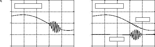
FIGURE 19-4

Example of single pole recursive filters. In (a), a high frequency burst rides on a slowly varying signal. In (b), single pole low-pass and high-pass filters are used to separate the two components. The low-pass filter uses x = 0.95, while the high-pass filter is for x = 0.86.

filter becomes unstable if x is made greater than one. That is, any nonzero value on the input will make the output increase until an overflow occurs.

The value for x can be directly specified, or found from the desired time constant of the filter. Just as R× C is the number of seconds it takes an RC circuit to decay to 36.8% of its final value, d is the number of samples it takes for a recursive filter to decay to this same level:

EQUATION 19-4

Time constant of single pole filters. This

equation relates the amount of decay x ' e & 1 /d between samples, x, with the filter's time

constant, d, the number of samples for the filter to decay to 36.8%.

For instance, a sample-to-sample decay of x ' 0.86 corresponds to a time constant of d ' 6.63 samples (as shown in Fig 19-3). There is also a fixed relationship between x and the -3dB cutoff frequency, fC , of the digital filter:

EQUATION 19-5

Cutoff frequency of single pole filters.

The amount of decay between samples, x, x ' e & 2 BfC is related to the cutoff frequency of the

filter, fC , a value between 0 and 0.5.

This provides three ways to find the "a" and "b" coefficients, starting with the time constant, the cutoff frequency, or just directly picking x.

Figure 19-4 shows an example of using single pole recursive filters. In (a), the original signal is a smooth curve, except a burst of a high frequency sine wave. Figure (b) shows the signal after passing through low-pass and high-pass filters. The signals have been separated fairly well, but not perfectly, just as if simple RC circuits were used on an analog signal.

Chapter 19Recursive Filters

325

1.5
	a. High-pass filter
1.0	0.01
Amplitude	0.05
0.5		fc = 0.25
0.0
0	0.1	0.2	0.3	0.4	0.5
		Frequency

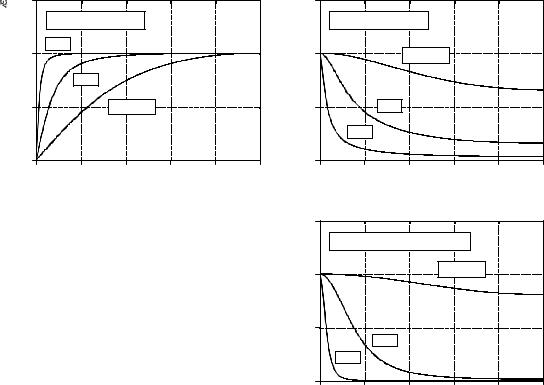
FIGURE 19-5

Single pole frequency responses. Figures (a) and (b) show the frequency responses of highpass and low-pass single pole recursive filters, respectively. Figure (c) shows the frequency response of a cascade of four low-pass filters. The frequency response of recursive filters is not always what you expect, especially if the filter is pushed to extreme limits. For example, the fC ' 0.25 curve in (c) is quite useless. Many factors are to blame, including: aliasing, roundoff noise, and the nonlinear phase response.

1.5
	b. Low-pass filter
1.0		fc = 0.25
Amplitude		0.05
0.5
	0.01
0.0
0	0.1	0.2	0.3	0.4	0.5
		Frequency
1.5

c. Low-pass filter (4 stage)

1.0			fc = 0.25
Amplitude
0.5
		0.05
	0.01
0.0
0	0.1	0.2	0.3	0.4	0.5

Frequency

Figure 19-5 shows the frequency responses of various single pole recursive filters. These curves are obtained by passing a delta function through the filter to find the filter's impulse response. The FFT is then used to convert the impulse response into the frequency response. In principle, the impulse response is infinitely long; however, it decays below the single precision roundoff noise after about 15 to 20 time constants. For example, when the time constant of the filter is d ' 6.63 samples, the impulse response can be contained in about 128 samples.

The key feature in Fig. 19-5 is that single pole recursive filters have little ability to separate one band of frequencies from another. In other words, they perform well in the time domain, and poorly in the frequency domain. The frequency response can be improved slightly by cascading several stages. This can be accomplished in two ways. First, the signal can be passed through the filter several times. Second, the z-transform can be used to find the recursion coefficients that combine the cascade into a single stage. Both ways work and are commonly used. Figure (c) shows the frequency response of a cascade of four low-pass filters. Although the stopband attenuation is significantly improved, the roll-off is still terrible. If you need better performance in the frequency domain, look at the Chebyshev filters of the next chapter.

326	The Scientist and Engineer's Guide to Digital Signal Processing

The four stage low-pass filter is comparable to the Blackman and Gaussian filters (relatives of the moving average, Chapter 15), but with a much faster execution speed. The design equations for a four stage low-pass filter are:

EQUATION 19-6

Four stage low-pass filter. These equations provide the "a" and "b" coefficients for a cascade of four single pole low-pass filters. The relationship between x and the cutoff frequency of this filter is given by Eq. 19-5, with the 2B replaced by 14.445.

a	0	'	(1& x )4
b1		'	4x
b	2	' & 6x 2
b	3	'	4x 3
b	4	' & x 4

Narrow-band Filters

A common need in electronics and DSP is to isolate a narrow band of frequencies from a wider bandwidth signal. For example, you may want to eliminate 60 hertz interference in an instrumentation system, or isolate the signaling tones in a telephone network. Two types of frequency responses are available: the band-pass and the band-reject (also called a notch filter). Figure 19-6 shows the frequency response of these filters, with the recursion coefficients provided by the following equations:

EQUATION 19-7

Band-pass filter. An example frequency response is shown in Fig. 19-6a. To use these equations, first select the center frequency, f, and the bandwidth, BW. Both of these are expressed as a fraction of the sampling rate, and therefore in the range of 0 to 0.5. Next, calculate R, and then K, and then the recursion coefficients.

EQUATION 19-8

Band-reject filter. This filter is commonly called a notch filter. Example frequency responses are shown in Fig. 19-6b.

	a0		'	1& K
	a1		'	2(K& R ) cos( 2Bf )
	a	2	'	R 2& K
				2R cos( 2Bf )
	b1		'
	b	2	'	& R 2
	a0		'	K
	a1		'	& 2K cos( 2Bf )
	a2		'	K
	b1		'	2R cos( 2Bf )
	b	2	'	& R 2
	where:
	K '			1 & 2R cos(2Bf ) % R 2
				2 & 2 cos(2Bf )
	R '			1 & 3 BW

Chapter 19Recursive Filters

327

1.5
	a. Band-pass frequency response
1.0
Amplitude
0.5	single stage
	BW=0.0066		cascade of
			three stages
0.0
0	0.1	0.2	0.3	0.4	0.5
		Frequency

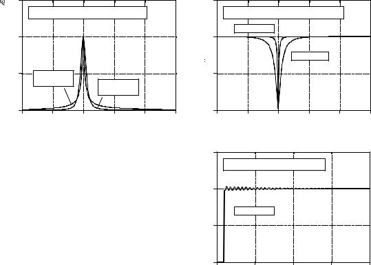
FIGURE 19-6

Characteristics of narrow-band filters. Figure (a) and (b) shows the frequency responses of various band-pass and band-reject filters. The step response of the band-reject filter is shown in (c). The band-reject (notch) filter is useful for removing 60 Hz and similar interference from time domain encoded waveforms.

Amplitude

Amplitude

1.5
	b. Band-reject frequency response
	BW=0.0066
1.0
			BW=0.033
0.5
0.0
0	0.1	0.2	0.3	0.4	0.5
		Frequency
1.5

c. Band-reject step response

1.0

BW=0.0066

0.5

0.0

0

50

100

150

200

Sample number

Two parameters must be selected before using these equations: f, the center frequency, and BW, the bandwidth (measured at an amplitude of 0.707). Both of these are expressed as a fraction of the sampling frequency, and therefore must be between 0 and 0.5. From these two specified values, calculate the intermediate variables: R and K, and then the recursion coefficients.

As shown in (a), the band-pass filter has relatively large tails extending from the main peak. This can be improved by cascading several stages. Since the design equations are quite long, it is simpler to implement this cascade by filtering the signal several times, rather than trying to find the coefficients needed for a single filter.

Figure (b) shows examples of the band-reject filter. The narrowest bandwidth that can be obtain with single precision is about 0.0003 of the sampling frequency. When pushed beyond this limit, the attenuation of the notch will degrade. Figure (c) shows the step response of the band-reject filter. There is noticeable overshoot and ringing, but its amplitude is quite small. This allows the filter to remove narrowband interference (60 Hz and the like) with only a minor distortion to the time domain waveform.

328	The Scientist and Engineer's Guide to Digital Signal Processing

Phase Response

There are three types of phase response that a filter can have: zero phase, linear phase, and nonlinear phase. An example of each of these is shown in Figure 19-7. As shown in (a), the zero phase filter is characterized by an impulse response that is symmetrical around sample zero. The actual shape doesn't matter, only that the negative numbered samples are a mirror image of the positive numbered samples. When the Fourier transform is taken of this symmetrical waveform, the phase will be entirely zero, as shown in (b).

The disadvantage of the zero phase filter is that it requires the use of negative indexes, which can be inconvenient to work with. The linear phase filter is a way around this. The impulse response in (d) is identical to that shown in (a), except it has been shifted to use only positive numbered samples. The impulse response is still symmetrical between the left and right; however, the location of symmetry has been shifted from zero. This shift results in the phase, (e), being a straight line, accounting for the name: linear phase. The slope of this straight line is directly proportional to the amount of the shift. Since the shift in the impulse response does nothing but produce an identical shift in the output signal, the linear phase filter is equivalent to the zero phase filter for most purposes.

Figure (g) shows an impulse response that is not symmetrical between the left and right. Correspondingly, the phase, (h), is not a straight line. In other words, it has a nonlinear phase. Don't confuse the terms: nonlinear and linear phase with the concept of system linearity discussed in Chapter 5. Although both use the word linear, they are not related.

Why does anyone care if the phase is linear or not? Figures (c), (f), and (i) show the answer. These are the pulse responses of each of the three filters. The pulse response is nothing more than a positive going step response followed by a negative going step response. The pulse response is used here because it displays what happens to both the rising and falling edges in a signal. Here is the important part: zero and linear phase filters have left and right edges that look the same, while nonlinear phase filters have left and right edges that look different. Many applications cannot tolerate the left and right edges looking different. One example is the display of an oscilloscope, where this difference could be misinterpreted as a feature of the signal being measured. Another example is in video processing. Can you imagine turning on your TV to find the left ear of your favorite actor looking different from his right ear?

It is easy to make an FIR (finite impulse response) filter have a linear phase. This is because the impulse response (filter kernel) is directly specified in the design process. Making the filter kernel have left-right symmetry is all that is required. This is not the case with IIR (recursive) filters, since the recursion coefficients are what is specified, not the impulse response. The impulse response of a recursive filter is not symmetrical between the left and right, and therefore has a nonlinear phase.