TsOS / DSP_guide_Smith / Ch6

CHAPTER

Convolution

6

Convolution is a mathematical way of combining two signals to form a third signal. It is the single most important technique in Digital Signal Processing. Using the strategy of impulse decomposition, systems are described by a signal called the impulse response. Convolution is important because it relates the three signals of interest: the input signal, the output signal, and the impulse response. This chapter presents convolution from two different viewpoints, called the input side algorithm and the output side algorithm. Convolution provides the mathematical framework for DSP; there is nothing more important in this book.

The Delta Function and Impulse Response

The previous chapter describes how a signal can be decomposed into a group of components called impulses. An impulse is a signal composed of all zeros, except a single nonzero point. In effect, impulse decomposition provides a way to analyze signals one sample at a time. The previous chapter also presented the fundamental concept of DSP: the input signal is decomposed into simple additive components, each of these components is passed through a linear system, and the resulting output components are synthesized (added). The signal resulting from this divide-and-conquer procedure is identical to that obtained by directly passing the original signal through the system. While many different decompositions are possible, two form the backbone of signal processing: impulse decomposition and Fourier decomposition. When impulse decomposition is used, the procedure can be described by a mathematical operation called convolution. In this chapter (and most of the following ones) we will only be dealing with discrete signals. Convolution also applies to continuous signals, but the mathematics is more complicated. We will look at how continious signals are processed in Chapter 13.

Figure 6-1 defines two important terms used in DSP. The first is the delta function, symbolized by the Greek letter delta, *[n]. The delta function is a normalized impulse, that is, sample number zero has a value of one, while

107

108 The Scientist and Engineer's Guide to Digital Signal Processing

all other samples have a value of zero. For this reason, the delta function is frequently called the unit impulse.

The second term defined in Fig. 6-1 is the impulse response. As the name suggests, the impulse response is the signal that exits a system when a delta function (unit impulse) is the input. If two systems are different in any way, they will have different impulse responses. Just as the input and output signals are often called x[n] and y[n] , the impulse response is usually given the symbol, h[n]. Of course, this can be changed if a more descriptive name is available, for instance, f [n] might be used to identify the impulse response of a filter.

Any impulse can be represented as a shifted and scaled delta function. Consider a signal, a[n] , composed of all zeros except sample number 8, which has a value of -3. This is the same as a delta function shifted to the r i g h t b y 8 s a m p l e s , a n d m u l t i p l i e d b y - 3 . I n e q u a t i o n f o r m : a[n] ' & 3*[n& 8]. Make sure you understand this notation, it is used in nearly all DSP equations.

If the input to a system is an impulse, such as & 3*[n& 8] , what is the system's output? This is where the properties of homogeneity and shift invariance are used. Scaling and shifting the input results in an identical scaling and shifting of the output. If *[n] results in h[n] , it follows that & 3*[n& 8] results in & 3h[n& 8] . In words, the output is a version of the impulse response that has been shifted and scaled by the same amount as the delta function on the input. If you know a system's impulse response, you immediately know how it will react to any impulse.

Convolution

Let's summarize this way of understanding how a system changes an input signal into an output signal. First, the input signal can be decomposed into a set of impulses, each of which can be viewed as a scaled and shifted delta function. Second, the output resulting from each impulse is a scaled and shifted version of the impulse response. Third, the overall output signal can be found by adding these scaled and shifted impulse responses. In other words, if we know a system's impulse response, then we can calculate what the output will be for any possible input signal. This means we know everything about the system. There is nothing more that can be learned about a linear system's characteristics. (However, in later chapters we will show that this information can be represented in different forms).

The impulse response goes by a different name in some applications. If the system being considered is a filter, the impulse response is called the filter kernel, the convolution kernel, or simply, the kernel. In image processing, the impulse response is called the point spread function. While these terms are used in slightly different ways, they all mean the same thing, the signal produced by a system when the input is a delta function.

Chapter 6- Convolution

109

									Delta																																					Impulse
						Function																																				Response
2																																					2
1																																					1
0																																					0
-1																																					-1
-2 -1 0 1 2 3 4 5 6																																					-2 -1 0 1 2 3 4 5 6
																				*[n]																Linear			h[n]
																																				System

FIGURE 6-1

Definition of delta function and impulse response. The delta function is a normalized impulse. All of its samples have a value of zero, except for sample number zero, which has a value of one. The Greek letter delta, *[n] , is used to identify the delta function. The impulse response of a linear system, usually denoted by h[n] , is the output of the system when the input is a delta function.

Convolution is a formal mathematical operation, just as multiplication, addition, and integration. Addition takes two numbers and produces a third number, while convolution takes two signals and produces a third signal. Convolution is used in the mathematics of many fields, such as probability and statistics. In linear systems, convolution is used to describe the relationship between three signals of interest: the input signal, the impulse response, and the output signal.

Figure 6-2 shows the notation when convolution is used with linear systems. An input signal, x[n] , enters a linear system with an impulse response, h[n] , resulting in an output signal, y[n] . In equation form: x[n] t h[n] ' y[n] . Expressed in words, the input signal convolved with the impulse response is equal to the output signal. Just as addition is represented by the plus, +, and multiplication by the cross, ×, convolution is represented by the star, t. It is unfortunate that most programming languages also use the star to indicate multiplication. A star in a computer program means multiplication, while a star in an equation means convolution.

FIGURE 6-2							Linear
How convolution is used in DSP. The
output signal from a linear system is	x[n]					System			y[n]
equal to the input signal convolved							h[n]
with the system's impulse response.
Convolution is denoted by a star when
writing equations.		x[n]					h[n] = y[n]

110	The Scientist and Engineer's Guide to Digital Signal Processing

a. Low-pass Filter
	4										0.08					4
	3										0.06					3
Amplitude										Amplitude					Amplitude
	2										0.04					2
	1															1
	0										0.02					0
	-1										0.00					-1
	-2										-0.02					-2
	0	10	20	30	40	50	60	70	80		0	10	20	30		0	10	20	30	40	50	60	70	80	90	100	110

Sample number

Sample Snumber

Sample number

b. High-pass Filter
	4										1.25					4
Amplitude	3									Amplitude	1.00				Amplitude	3
	2										0.75					2
	1										0.50					1
	0										0.25					0
	-1										0.00					-1
	-2										-0.25					-2
	0	10	20	30	40	50	60	70	80		0	10	20	30		0	10	20	30	40	50	60	70	80	90	100	110

Sample number	SampleSnumber	Sample number
Input Signal	Impulse Response	Output Signal

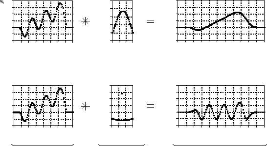
FIGURE 6-3

Examples of low-pass and high-pass filtering using convolution. In this example, the input signal is a few cycles of a sine wave plus a slowly rising ramp. These two components are separated by using properly selected impulse responses.

Figure 6-3 shows convolution being used for low-pass and high-pass filtering. The example input signal is the sum of two components: three cycles of a sine wave (representing a high frequency), plus a slowly rising ramp (composed of low frequencies). In (a), the impulse response for the low-pass filter is a smooth arch, resulting in only the slowly changing ramp waveform being passed to the output. Similarly, the high-pass filter, (b), allows only the more rapidly changing sinusoid to pass.

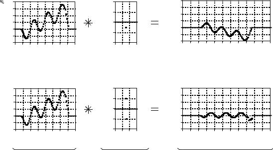
Figure 6-4 illustrates two additional examples of how convolution is used to process signals. The inverting attenuator, (a), flips the signal top-for-bottom, and reduces its amplitude. The discrete derivative (also called the first difference), shown in (b), results in an output signal related to the slope of the input signal.

Notice the lengths of the signals in Figs. 6-3 and 6-4. The input signals are 81 samples long, while each impulse response is composed of 31 samples. In most DSP applications, the input signal is hundreds, thousands, or even millions of samples in length. The impulse response is usually much shorter, say, a few points to a few hundred points. The mathematics behind convolution doesn't restrict how long these signals are. It does, however, specify the length of the output signal. The length of the output signal is

Chapter 6- Convolution

111

a. Inverting Attenuator
	4										2.00					4
	3															3
											1.00
Amplitude	2									Amplitude					Amplitude	2
	1										0.00					1
	0															0
											-1.00
	-1															-1
	-2										-2.00					-2
																0	10	20	30	40	50	60	70	80	90	100	110
	0	10	20	30	40	50	60	70	80		0	10	20	30
																				Sample number
			Sample number								Sample Snumber

b. Discrete Derivative

	4										2.00					4
	3										1.00					3
Amplitude	2									Amplitude					Amplitude	2
	1										0.00					1
	0										-1.00					0
	-1															-1
	-2										-2.00					-2
	0	10	20	30	40	50	60	70	80		0	10	20	30		0	10	20	30	40	50	60	70	80	90	100	110

Sample number	Sample Snumber	Sample number
Input Signal	Impulse Response	Output Signal

FIGURE 6-4

Examples of signals being processed using convolution. Many signal processing tasks use very simple impulse responses. As shown in these examples, dramatic changes can be achieved with only a few nonzero points.

equal to the length of the input signal, plus the length of the impulse response, minus one. For the signals in Figs. 6-3 and 6-4, each output signal is: 81 % 31 & 1 ' 111 samples long. The input signal runs from sample 0 to 80, the impulse response from sample 0 to 30, and the output signal from sample 0 to 110.

Now we come to the detailed mathematics of convolution. As used in Digital Signal Processing, convolution can be understood in two separate ways. The first looks at convolution from the viewpoint of the input signal. This involves analyzing how each sample in the input signal contributes to many points in the output signal. The second way looks at convolution from the viewpoint of the output signal. This examines how each sample in the output signal has received information from many points in the input signal.

Keep in mind that these two perspectives are different ways of thinking about the same mathematical operation. The first viewpoint is important because it provides a conceptual understanding of how convolution pertains to DSP. The second viewpoint describes the mathematics of convolution. This typifies one of the most difficult tasks you will encounter in DSP: making your conceptual understanding fit with the jumble of mathematics used to communicate the ideas.

112	The Scientist and Engineer's Guide to Digital Signal Processing

The Input Side Algorithm

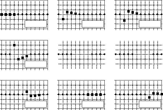
Figure 6-5 shows a simple convolution problem: a 9 point input signal, x[n] , is passed through a system with a 4 point impulse response, h[n] , resulting in a 9 % 4 & 1 ' 12 point output signal, y[n] . In mathematical terms, x[n] is convolved with h[n] to produce y[n] . This first viewpoint of convolution is based on the fundamental concept of DSP: decompose the input, pass the components through the system, and synthesize the output. In this example, each of the nine samples in the input signal will contribute a scaled and shifted version of the impulse response to the output signal. These nine signals are shown in Fig. 6-6. Adding these nine signals produces the output signal, y[n] .

Let's look at several of these nine signals in detail. We will start with sample number four in the input signal, i.e., x[4] . This sample is at index number four, and has a value of 1.4. When the signal is decomposed, this turns into an impulse represented as: 1.4 *[n& 4]. After passing through the system, the resulting output component will be: 1.4 h[n& 4]. This signal is shown in the center box of the nine signals in Fig. 6-6. Notice that this is the impulse response, h[n] , multiplied by 1.4, and shifted four samples to the right. Zeros have been added at samples 0-3 and at samples 8-11 to serve as place holders. To make this more clear, Fig. 6-6 uses squares to represent the data points that come from the shifted and scaled impulse response, and diamonds for the added zeros.

Now examine sample x[8] , the last point in the input signal. This sample is at index number eight, and has a value of -0.5. As shown in the lower-right graph of Fig. 6-6, x[8] results in an impulse response that has been shifted to the right by eight points and multiplied by -0.5. Place holding zeros have been added at points 0-7. Lastly, examine the effect of points x[0] and x[7] . Both these samples have a value of zero, and therefore produce output components consisting of all zeros.

			x[n]														h[n]									y[n]
3													3						3
2													2						2
1													1						1
0															0						0

-1	-1	-1
-2	-2	-2

-3																					-3								-3
0		1		2		3		4			5			6			7		8		0		1		2		3		0		1			2			3		4		5		6			7			8			9		10 11

FIGURE 6-5

Example convolution problem. A nine point input signal, convolved with a four point impulse response, results in a twelve point output signal. Each point in the input signal contributes a scaled and shifted impulse response to the output signal. These nine scaled and shifted impulse responses are shown in Fig. 6-6.

Chapter 6- Convolution

113

3											3											3
2											2											2
1											1											1
0											0											0
-1											-1											-1
-2						contribution					-2						contribution					-2						contribution
						from		x[0] h[n- 0]									from		x[1] h[n- 1]									from		x[2] h[n- 2]
-3											-3											-3
0	1	2	3	4	5	6	7	8	9	10 11	0	1	2	3	4	5	6	7	8	9	10 11	0	1	2	3	4	5	6	7	8	9	10 11

	3
	2
	1
	0
	-1
	-2	contribution
		from	x[ 3] h[n- 3]
	-3

3																											3
2																											2
1																											1
0																											0
-1																											-1
-2												contribution															-2													contribution
												from x[4] h[n- 4]																												from x[5] h[n- 5]
-3																											-3

0	1	2	3	4	5	6	7	8	9	10 11	0	1	2	3	4	5	6	7	8	9	10 11	0	1	2	3	4	5	6	7	8	9	10 11
3											3											3
2											2											2
1											1											1
0											0											0
-1											-1											-1
-2						contribution					-2						contribution					-2						contribution
						from		x[6] h[n- 6]									from		x[7] h[n- 7]									from		x[8] h[n- 8]
-3											-3											-3
0	1	2	3	4	5	6	7	8	9	10 11	0	1	2	3	4	5	6	7	8	9	10 11	0	1	2	3	4	5	6	7	8	9	10 11

FIGURE 6-6

Output signal components for the convolution in Fig. 6-5. In these signals, each point that results from a scaled and shifted impulse response is represented by a square marker. The remaining data points, represented by diamonds, are zeros that have been added as place holders.

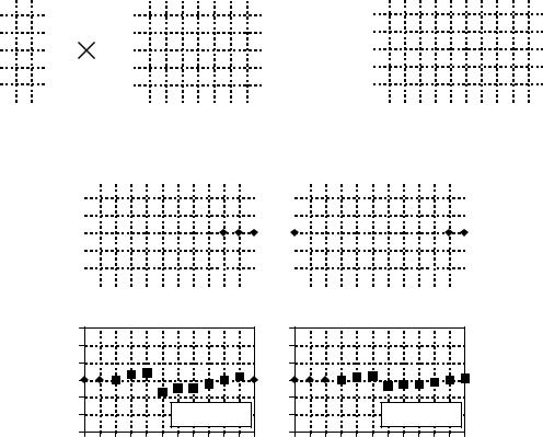
In this example, x[n] is a nine point signal and h[n] is a four point signal. In our next example, shown in Fig. 6-7, we will reverse the situation by making x[n] a four point signal, and h[n] a nine point signal. The same two waveforms are used, they are just swapped. As shown by the output signal components, the four samples in x[n] result in four shifted and scaled versions of the nine point impulse response. Just as before, leading and trailing zeros are added as place holders.

But wait just one moment! The output signal in Fig. 6-7 is identical to the output signal in Fig. 6-5. This isn't a mistake, but an important property. Convolution is commutative: a[n] tb[n] ' b[n] ta[n] . The mathematics does not care which is the input signal and which is the impulse response, only that two signals are convolved with each other. Although the mathematics may allow it, exchanging the two signals has no physical meaning in system theory. The input signal and impulse response are two totally different things and exchanging them doesn't make sense. What the commutative property provides is a mathematical tool for manipulating equations to achieve various results.

114	The Scientist and Engineer's Guide to Digital Signal Processing

A program for calculating convolutions using the input side algorithm is shown in Table 6-1. Remember, the programs in this book are meant to convey algorithms in the simplest form, even at the expense of good programming style. For instance, all of the input and output is handled in mythical subroutines (lines 160 and 280), meaning we do not define how these operations are conducted. Do not skip over these programs; they are a key part of the material and you need to understand them in detail.

The program convolves an 81 point input signal, held in array X[ ], with a 31 point impulse response, held in array H[ ], resulting in a 111 point output signal, held in array Y[ ]. These are the same lengths shown in Figs. 6-3 and 6-4. Notice that the names of these arrays use upper case letters. This is a violation of the naming conventions previously discussed, because upper case letters are reserved for frequency domain signals. Unfortunately, the simple BASIC used in this book does not allow lower case variable names. Also notice that line 240 uses a star for multiplication. Remember, a star in a program means multiplication, while a star in an equation means convolution. A star in text (such as documentation or program comments) can mean either.

The mythical subroutine in line 160 places the input signal into X[ ] and the impulse response into H[ ]. Lines 180-200 set all of the values in Y[ ] to zero. This is necessary because Y[ ] is used as an accumulator to sum the output components as they are calculated. Lines 220 to 260 are the heart of the program. The FOR statement in line 220 controls a loop that steps through each point in the input signal, X[ ]. For each sample in the input signal, an inner loop (lines 230-250) calculates a scaled and shifted version of the impulse response, and adds it to the array accumulating the output signal, Y[ ]. This nested loop structure (one loop within another loop) is a key characteristic of convolution programs; become familiar with it.

100	'CONVOLUTION USING THE INPUT SIDE ALGORITHM
110		'
120	DIM X[80]	'The input signal, 81 points
130	DIM H[30]	'The impulse response, 31 points
140	DIM Y[110]	'The output signal, 111 points
150		'
160	GOSUB XXXX	'Mythical subroutine to load X[ ] and H[ ]
170		'
180	FOR I% = 0 TO 110	'Zero the output array
190	Y(I%) = 0
200 NEXT I%
210		'
220	FOR I% = 0 TO 80	'Loop for each point in X[ ]
230	FOR J% = 0 TO 30 'Loop for each point in H[ ]
240	Y[I%+J%] = Y[I%+J%] + X[I%]tH[J%]
250	NEXT J%
260 NEXT I%		'(remember, t is multiplication in programs!)
270		'
280	GOSUB XXXX	'Mythical subroutine to store Y[ ]
290		'

300 END

TABLE 6-1

																																	Chapter 6- Convolution																																																115
	x[n]																										h[n]																																													y[n]
3													3																																				3
2													2																																				2
1													1																																				1
0																	0																																						0
-1																-1																																	-1
-2													-2																																				-2
-3													-3																																				-3
0		1				2					3		0											1	2	3						4	5					6	7						8				0																	1		2	3	4				5		6		7	8	9	10 11
																										Output signal components
													3																																				3
													2																																				2
													1																																				1
													0																																				0
													-1																																				-1
													-2														contribution																						-2																			contribution
																											from						x[0] h[n- 0]																																			from	x[1] h[n- 1]
													-3																																				-3

0	1	2	3	4	5	6	7	8	9	10 11	0	1	2	3	4	5	6	7	8	9	10 11
3											3
2											2
1											1
0											0
-1											-1
-2						contribution					-2						contribution
						from		x[ 2] h[n- 2]									from		x[3] h[n- 3]
-3											-3
0	1	2	3	4	5	6	7	8	9	10 11	0	1	2	3	4	5	6	7	8	9	10 11

FIGURE 6-7

A second example of convolution. The waveforms for the input signal and impulse response are exchanged from the example of Fig. 6-5. Since convolution is commutative, the output signals for the two examples are identical.

Keeping the indexing straight in line 240 can drive you crazy! Let's say we are halfway through the execution of this program, so that we have just begun action on sample X[40], i.e., I% = 40. The inner loop runs through each point in the impulse response doing three things. First, the impulse response is scaled by multiplying it by the value of the input sample. If this were the only action taken by the inner loop, line 240 could be written, Y[J%] = X[40]tH[J%]. Second, the scaled impulse is shifted 40 samples to the right by adding this number to the index used in the output signal. This second action would change line 240 to: Y[40+J%] = X[40]tH[J%]. Third, Y[ ] must accumulate (synthesize) all the signals resulting from each sample in the input signal. Therefore, the new information must be added to the information that is already in the array. This results in the final command: Y[40+J%] = Y[40+J%] + X[40]tH[J%]. Study this carefully; it is very confusing, but very important.

116	The Scientist and Engineer's Guide to Digital Signal Processing

The Output Side Algorithm

The first viewpoint of convolution analyzes how each sample in the input signal affects many samples in the output signal. In this second viewpoint, we reverse this by looking at individual samples in the output signal, and finding the contributing points from the input. This is important from both mathematical and practical standpoints. Suppose that we are given some input signal and impulse response, and want to find the convolution of the two. The most straightforward method would be to write a program that loops through the output signal, calculating one sample on each loop cycle. Likewise, equations are written in the form: y[n] ' some combination of other variables. That is, sample n in the output signal is equal to some combination of the many values in the input signal and impulse response. This requires a knowledge of how each sample in the output signal can be calculated independently of all other samples in the output signal. The output side algorithm provides this information.

Let's look at an example of how a single point in the output signal is influenced by several points from the input. The example point we will use is y[6] in Fig. 6-5. This point is equal to the sum of all the sixth points in the nine output components, shown in Fig. 6-6. Now, look closely at these nine output components and identify which can affect y[6] . That is, find which of these nine signals contains a nonzero sample at the sixth position. Five of the output components only have added zeros (the diamond markers) at the sixth sample, and can therefore be ignored. Only four of the output components are capable of having a nonzero value in the sixth position. These are the output components generated from the input samples: x[3], x[4], x[5], and x[6] . By adding the sixth sample from each of these output components, y[6] is determined as: y[6] ' x[3] h[3] % x[4 ]h[2] % x[5] h[1] % x[6]h[0] . That is, four samples from the input signal are multiplied by the four samples in the impulse response, and the products added.

Figure 6-8 illustrates the output side algorithm as a convolution machine, a flow diagram of how convolution occurs. Think of the input signal, x[n] , and the output signal, y[n] , as fixed on the page. The convolution machine, everything inside the dashed box, is free to move left and right as needed. The convolution machine is positioned so that its output is aligned with the output sample being calculated. Four samples from the input signal fall into the inputs of the convolution machine. These values are multiplied by the indicated samples in the impulse response, and the products are added. This produces the value for the output signal, which drops into its proper place. For example, y[6] i s s h o w n b e i n g c a l c u l a t e d f r o m t h e f o u r i n p u t s a m p l e s : x[3], x[4], x[5], and x[6] .

To calculate y[7] , the convolution machine moves one sample to the right. This results in another four samples entering the machine, x[4] through x[7] , and the value for y[7] dropping into the proper place. This process is repeated for all points in the output signal needing to be calculated.