TsOS / DSP_guide_Smith / Ch21

CHAPTER

Filter Comparison

21

Decisions, decisions, decisions! With all these filters to choose from, how do you know which to use? This chapter is a head-to-head competition between filters; we'll select champions from each side and let them fight it out. In the first match, digital filters are pitted against analog filters to see which technology is best. In the second round, the windowed-sinc is matched against the Chebyshev to find the king of the frequency domain filters. In the final battle, the moving average fights the single pole filter for the time domain championship. Enough talk; let the competition begin!

Match #1: Analog vs. Digital Filters

Most digital signals originate in analog electronics. If the signal needs to be filtered, is it better to use an analog filter before digitization, or a digital filter after? We will answer this question by letting two of the best contenders deliver their blows.

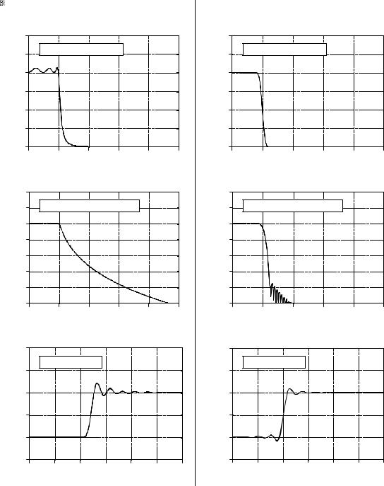
The goal will be to provide a low-pass filter at 1 kHz. Fighting for the analog side is a six pole Chebyshev filter with 0.5 dB (6%) ripple. As described in Chapter 3, this can be constructed with 3 op amps, 12 resistors, and 6 capacitors. In the digital corner, the windowed-sinc is warming up and ready to fight. The analog signal is digitized at a 10 kHz sampling rate, making the cutoff frequency 0.1 on the digital frequency scale. The length of the windowed-sinc will be chosen to be 129 points, providing the same 90% to 10% roll-off as the analog filter. Fair is fair. Figure 21-1 shows the frequency and step responses for these two filters.

Let's compare the two filters blow-by-blow. As shown in (a) and (b), the analog filter has a 6% ripple in the passband, while the digital filter is perfectly flat (within 0.02%). The analog designer might argue that the ripple can be selected in the design; however, this misses the point. The flatness achievable with analog filters is limited by the accuracy of their resistors and

343

344	The Scientist and Engineer's Guide to Digital Signal Processing

capacitors. Even if a Butterworth response is designed (i.e., 0% ripple), filters of this complexity will have a residue ripple of, perhaps, 1%. On the other hand, the flatness of digital filters is primarily limited by round-off error, making them hundreds of times flatter than their analog counterparts. Score one point for the digital filter.

Next, look at the frequency response on a log scale, as shown in (c) and (d). Again, the digital filter is clearly the victor in both roll-off and stopband attenuation. Even if the analog performance is improved by adding additional stages, it still can't compare to the digital filter. For instance, imagine that you need to improve these two parameters by a factor of 100. This can be done with simple modifications to the windowed-sinc, but is virtually impossible for the analog circuit. Score two more for the digital filter.

The step response of the two filters is shown in (e) and (f). The digital filter's step response is symmetrical between the lower and upper portions of the step, i.e., it has a linear phase. The analog filter's step response is not symmetrical, i.e., it has a nonlinear phase. One more point for the digital filter. Lastly, the analog filter overshoots about 20% on one side of the step. The digital filter overshoots about 10%, but on both sides of the step. Since both are bad, no points are awarded.

In spite of this beating, there are still many applications where analog filters should, or must, be used. This is not related to the actual performance of the filter (i.e., what goes in and what comes out), but to the general advantages that analog circuits have over digital techniques. The first advantage is speed: digital is slow; analog is fast. For example, a personal computer can only filter data at about 10,000 samples per second, using FFT convolution. Even simple op amps can operate at 100 kHz to 1 MHz, 10 to 100 times as fast as the digital system!

The second inherent advantage of analog over digital is dynamic range. This comes in two flavors. Amplitude dynamic range is the ratio between the largest signal that can be passed through a system, and the inherent noise of the system. For instance, a 12 bit ADC has a saturation level of 4095, and an rms quantization noise of 0.29 digital numbers, for a dynamic range of about 14000. In comparison, a standard op amp has a saturation voltage of about 20 volts and an internal noise of about 2 microvolts, for a dynamic range of about ten million. Just as before, a simple op amp devastates the digital system.

The other flavor is frequency dynamic range. For example, it is easy to design an op amp circuit to simultaneously handle frequencies between 0.01 Hz and 100 kHz (seven decades). When this is tried with a digital system, the computer becomes swamped with data. For instance, sampling at 200 kHz, it takes 20 million points to capture one complete cycle at 0.01 Hz. You may have noticed that the frequency response of digital filters is almost always plotted on a linear frequency scale, while analog filters are usually displayed with a logarithmic frequency. This is because digital filters need

Chapter 21Filter Comparison

345

		Analog Filter
	(6 pole 0.5dB Chebyshev)
1.50
1.25	a. Frequency response
1.00
Amplitude
0.75
0.50
0.25
0.00
0	1000	2000	3000	4000	5000

Frequency (hertz)

	40
	20	c. Frequency response (dB)
(dB)	0
	-20
Amplitude
	-40
	-60
	-80
	-100
	0	1000	2000	3000	4000	5000

Frequency (hertz)

	2.0
		e. Step response
Amplitude	1.5
	1.0
	0.5
	0.0
	-0.5
	-4	-2	0	2	4	6	8

Time (milliseconds)

Digital Filter

(129 point windowed-sinc)

	1.50
	1.25	b. Frequency response
Amplitude	1.00
	0.75
	0.50
	0.25
	0.00
	0	0.1	0.2	0.3		0.4	0.5
			Frequency
	40
	20	d. Frequency response (dB)
(dB)	0
	-20
Amplitude
	-40
	-60
	-80
	-100
	0	0.1	0.2	0.3		0.4	0.5
			Frequency
	2.0
		f. Step response
	1.5
Amplitude	1.0
	0.5
	0.0
	-0.5
	-40	-20	0	20	40	60	80

Sample number

FIGURE 21-1

Comparison of analog and digital filters. Digital filters have better performance in many areas, such as: passband ripple, (a) vs. (b), roll-off and stopband attenuation, (c) vs. (d), and step response symmetry,

(e) vs. (f). The digital filter in this example has a cutoff frequency of 0.1 of the 10 kHz sampling rate. This provides a fair comparison to the 1 kHz cutoff frequency of the analog filter.

a linear scale to show their exceptional filter performance, while analog filters need the logarithmic scale to show their huge dynamic range.

346	The Scientist and Engineer's Guide to Digital Signal Processing

Match #2: Windowed-Sinc vs. Chebyshev

Both the windowed-sinc and the Chebyshev filters are designed to separate one band of frequencies from another. The windowed-sinc is an FIR filter implemented by convolution, while the Chebyshev is an IIR filter carried out by recursion. Which is the best digital filter in the frequency domain? We'll let them fight it out.

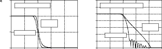
The recursive filter contender will be a 0.5% ripple, 6 pole Chebyshev low-pass filter. A fair comparison is complicated by the fact that the Chebyshev's frequency response changes with the cutoff frequency. We will use a cutoff frequency of 0.2, and select the windowed-sinc's filter kernel to be 51 points. This makes both filters have the same 90% to 10% roll-off, as shown in Fig. 21-2(a).

Now the pushing and shoving begins. The recursive filter has a 0.5% ripple in the passband, while the windowed-sinc is flat. However, we could easily set the recursive filter ripple to 0% if needed. No points. Figure 21-2b shows that the windowed-sinc has a much better stopband attenuation than the Chebyshev. One point for the windowed-sinc.

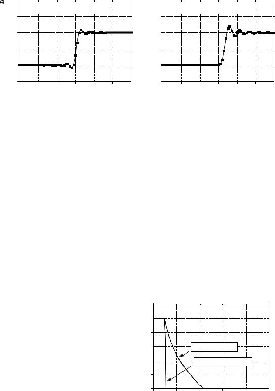
Figure 21-3 shows the step response of the two filters. Both are bad, as you should expect for frequency domain filters. The recursive filter has a nonlinear phase, but this can be corrected with bidirectional filtering. Since both filters are so ugly in this parameter, we will call this a draw.

So far, there isn't much difference between these two filters; either will work when moderate performance is needed. The heavy hitting comes over two critical issues: maximum performance and speed. The windowed-sinc is a powerhouse, while the Chebyshev is quick and agile. Suppose you have a really tough frequency separation problem, say, needing to isolate a 100

1.5
	a. Frequency response
1.0
Amplitude			Chebyshev
			recursive
0.5	windowed-sinc
0.0
0	0.1	0.2	0.3	0.4	0.5
		Frequency

	40
	20	b. Frequency response (dB)
(dB)	0
	-20
Amplitude
	-40				Chebyshev
					recursive
	-60	windowed-sinc
	-80
	-100
	0	0.1	0.2	0.3	0.4	0.5
			Frequency

FIGURE 21-2

Windowed-sinc and Chebyshev frequency responses. Frequency responses are shown for a 51 point windowed-sinc filter and a 6 pole, 0.5% ripple Chebyshev recursive filter. The windowed-sinc has better stopband attenuation, but either will work in moderate performance applications. The cutoff frequency of both filters is 0.2, measured at an amplitude of 0.5 for the windowed-sinc, and 0.707 for the recursive.

									Chapter 21Filter Comparison															347
2.0													2.0
		a.	Windowed-sinc step response												b. Chebyshev step response

Amplitude	1.5							Amplitude	1.5
	0.5								0.5
	1.0								1.0
	0.0								0.0
	-0.5								-0.5
	-30	-20	-10	0	10	20	30		-30	-20	-10	0	10	20	30
			Sample number								Sample number

FIGURE 21-3

Windowed--sinc and Chebyshev step responses. The step responses are shown for a 51 point windowed-sinc filter and a 6 pole, 0.5% ripple Chebyshev recursive filter. Each of these filters has a cutoff frequency of 0.2. The windowed-sinc has a slightly better step response because it has less overshoot and a zero phase.

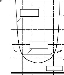
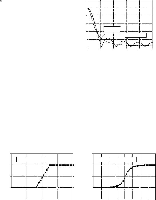
millivolt signal at 61 hertz that is riding on a 120 volt power line at 60 hertz. Figure 21-4 shows how these two filters compare when you need maximum performance. The recursive filter is a 6 pole Chebyshev with 0.5% ripple. This is the maximum number of poles that can be used at a 0.05 cutoff frequency with single precision. The windowed-sinc uses a 1001 point filter kernel, formed by convolving a 501 point windowed-sinc filter kernel with itself. As shown in Chapter 16, this provides greater stopband attenuation.

How do these two filters compare when maximum performance is needed? The windowed-sinc crushes the Chebyshev! Even if the recursive filter were improved (more poles, multistage implementation, double precision, etc.), it is still no match for the FIR performance. This is especially impressive when you consider that the windowed-sinc has only begun to fight. There are strong limits on the maximum performance that recursive filters can provide. The windowed-sinc, in contrast, can be pushed to incredible levels. This is, of course, provided you are willing to wait for the result. Which brings up the second critical issue: speed.

FIGURE 21-4

Maximum performance of FIR and IIR filters. The frequency response of the windowed-sinc can be virtually any shape needed, while the Chebyshev recursive filter is very limited. This graph compares the frequency response of a six pole Chebyshev recursive filter with a 1001 point windowed-sinc filter.

	20
	0
(dB)	-20
Amplitude	-40		Chebyshev (IIR)
	-60		Windowed-sinc (FIR)
	-80
	-100
	0	0.1	0.2	0.3	0.4	0.5
			Frequency

348	The Scientist and Engineer's Guide to Digital Signal Processing

FIGURE 21-5

Comparing FIR and IIR execution speeds. These curves shows the relative execution times for a windowed-sinc filter compared with an equivalent six pole Chebyshev recursive filter. Curves are shown for implementing the FIR filter by both the standard and the FFT convolution algorithms. The windowed-sinc execution time rises at low and high frequencies because the filter kernel must be made longer to keep up with the greater performance of the recursive filter at these frequencies. In general, IIR filters are an order of magnitude faster than FIR filters of comparable performance.

	50
		standard
	40	convolution
time
execution	30
Relative	20		FFT
			convolution
	10
					Recursive
	0
	0	0.1	0.2	0.3	0.4	0.5
			Frequency

Comparing these filters for speed is like racing a Ferrari against a go-cart. Figure 21-5 shows how much longer the windowed-sinc takes to execute, compared to a six pole recursive filter. Since the recursive filter has a faster roll-off at low and high frequencies, the length of the windowed-sinc kernel must be made longer to match the performance (i.e., to keep the comparison fair). This accounts for the increased execution time for the windowed-sinc near frequencies 0 and 0.5. The important point is that FIR filters can be expected to be about an order of magnitude slower than comparable IIR filters (go-cart: 15 mph, Ferrari: 150 mph).

Match #3: Moving Average vs. Single Pole

Our third competition will be a battle of the time domain filters. The first fighter will be a nine point moving average filter. Its opponent for today's match will be a single pole recursive filter using the bidirectional technique. To achieve a comparable frequency response, the single pole filter will use a sample-to-sample decay of x ' 0.70 . The battle begins in Fig. 21-6 where the frequency response of each filter is shown. Neither one is very impressive, but of course, frequency separation isn't what these filters are used for. No points for either side.

Figure 21-7 shows the step responses of the filters. In (a), the moving average step response is a straight line, the most rapid way of moving from one level to another. In (b), the recursive filter's step response is smoother, which may be better for some applications. One point for each side.

These filters are quite equally matched in terms of performance and often the choice between the two is made on personal preference. However, there are

Chapter 21Filter Comparison

349

FIGURE 21-6

Moving average and single pole frequency responses. Both of these filters have a poor frequency response, as you should expect for time domain filters.

	1.2
	1.0
Amplitude	0.8
	0.6		Single pole
	0.4		recursive
				Moving average
	0.2
	0.0
	0	0.1	0.2	0.3	0.4	0.5
			Frequency

two cases where one filter has a slight edge over the other. These are based on the trade-off between development time and execution time. In the first instance, you want to reduce development time and are willing to accept a slower filter. For example, you might have a one time need to filter a few thousand points. Since the entire program runs in only a few seconds, it is pointless to spend time optimizing the algorithm. Floating point will almost certainly be used. The choice is to use the moving average filter carried out by convolution, or a single pole recursive filter. The winner here is the recursive filter. It will be slightly easier to program and modify, and will execute much faster.

The second case is just the opposite; your filter must operate as fast as possible and you are willing to spend the extra development time to get it. For instance, this filter might be a part of a commercial product, with the potential to be run millions of times. You will probably use integers for the highest possible speed. Your choice of filters will be the moving average

		1.5		1.5
		a. Moving average		b. Bidirectional recursive
	Amplitude	1.0	Amplitude	1.0
		0.5		0.5

0.0															0.0
-0.5															-0.5
-20			-10			0			10				20		-20 -15 -10							-5		0		5			10				15			20
						Sample number																Sample number

FIGURE 21-7

Step responses of the moving average and the bidirectional single pole filter. The moving average step response occurs over a smaller number of samples, while the single pole filter's step response is smoother.

350	The Scientist and Engineer's Guide to Digital Signal Processing

carried out by recursion, or the single pole recursive filter implemented with look-up tables or integer math. The winner is the moving average filter. It will execute faster and not be susceptible to the development and execution problems of integer arithmetic.