CHAPTER

Linear Image Processing

24

Linear image processing is based on the same two techniques as conventional DSP: convolution and Fourier analysis. Convolution is the more important of these two, since images have their information encoded in the spatial domain rather than the frequency domain. Linear filtering can improve images in many ways: sharpening the edges of objects, reducing random noise, correcting for unequal illumination, deconvolution to correct for blur and motion, etc. These procedures are carried out by convolving the original image with an appropriate filter kernel, producing the filtered image. A serious problem with image convolution is the enormous number of calculations that need to be performed, often resulting in unacceptably long execution times. This chapter presents strategies for designing filter kernels for various image processing tasks. Two important techniques for reducing the execution time are also described: convolution by separability and

FFT convolution.

Convolution

Image convolution works in the same way as one-dimensional convolution. For instance, images can be viewed as a summation of impulses, i.e., scaled and shifted delta functions. Likewise, linear systems are characterized by how they respond to impulses; that is, by their impulse responses. As you should expect, the output image from a system is equal to the input image convolved with the system's impulse response.

The two-dimensional delta function is an image composed of all zeros, except for a single pixel at: row = 0, column = 0, which has a value of one. For now, assume that the row and column indexes can have both positive and negative values, such that the one is centered in a vast sea of zeros. When the delta function is passed through a linear system, the single nonzero point will be changed into some other two-dimensional pattern. Since the only thing that can happen to a point is that it spreads out, the impulse response is often called the point spread function (PSF) in image processing jargon.

397

398	The Scientist and Engineer's Guide to Digital Signal Processing

The human eye provides an excellent example of these concepts. As described in the last chapter, the first layer of the retina transforms an image represented as a pattern of light into an image represented as a pattern of nerve impulses. The second layer of the retina processes this neural image and passes it to the third layer, the fibers forming the optic nerve. Imagine that the image being projected onto the retina is a very small spot of light in the center of a dark background. That is, an impulse is fed into the eye. Assuming that the system is linear, the image processing taking place in the retina can be determined by inspecting the image appearing at the optic nerve. In other words, we want to find the point spread function of the processing. We will revisit the assumption about linearity of the eye later in this chapter.

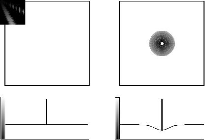
Figure 24-1 outlines this experiment. Figure (a) illustrates the impulse striking the retina while (b) shows the image appearing at the optic nerve. The middle layer of the eye passes the bright spike, but produces a circular region of increased darkness. The eye accomplishes this by a process known as lateral inhibition. If a nerve cell in the middle layer is activated, it decreases the ability of its nearby neighbors to become active. When a complete image is viewed by the eye, each point in the image contributes a scaled and shifted version of this impulse response to the image appearing at the optic nerve. In other words, the visual image is convolved with this PSF to produce the neural image transmitted to the brain. The obvious question is: how does convolving a viewed image with this PSF improve the ability of the eye to understand the world?

a. Image at first layer		b. Image at third layer

FIGURE 24-1

The PSF of the eye. The middle layer of the retina changes an impulse, shown in (a), into an impulse surrounded by a dark area, shown in (b). This point spread function enhances the edges of objects.

Chapter 24Linear Image Processing

399

a. True brightness

FIGURE 24-2

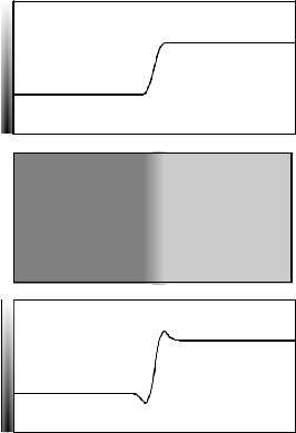
Mach bands. Image processing in the retina results in a slowly changing edge, as in (a), being sharpened, as in (b). This makes it easier to separate objects in the image, but produces an optical illusion called Mach bands. Near the edge, the overshoot makes the dark region look darker, and the light region look lighter. This produces dark and light bands that run parallel to the edge.

b. Perceived brightness

Humans and other animals use vision to identify nearby objects, such as enemies, food, and mates. This is done by distinguishing one region in the image from another, based on differences in brightness and color. In other words, the first step in recognizing an object is to identify its edges, the discontinuity that separates an object from its background. The middle layer of the retina helps this task by sharpening the edges in the viewed image. As an illustration of how this works, Fig. 24-2 shows an image that slowly changes from dark to light, producing a blurry and poorly defined edge. Figure

(a) shows the intensity profile of this image, the pattern of brightness entering the eye. Figure (b) shows the brightness profile appearing on the optic nerve, the image transmitted to the brain. The processing in the retina makes the edge between the light and dark areas appear more abrupt, reinforcing that the two regions are different.

The overshoot in the edge response creates an interesting optical illusion. Next to the edge, the dark region appears to be unusually dark, and the light region appears to be unusually light. The resulting light and dark strips are called Mach bands, after Ernst Mach (1838-1916), an Austrian physicist who first described them.

As with one-dimensional signals, image convolution can be viewed in two ways: from the input, and from the output. From the input side, each pixel in

400	The Scientist and Engineer's Guide to Digital Signal Processing

the input image contributes a scaled and shifted version of the point spread function to the output image. As viewed from the output side, each pixel in the output image is influenced by a group of pixels from the input signal. For one-dimensional signals, this region of influence is the impulse response flipped left-for-right. For image signals, it is the PSF flipped left-for-right and top- for-bottom. Since most of the PSFs used in DSP are symmetrical around the vertical and horizonal axes, these flips do nothing and can be ignored. Later in this chapter we will look at nonsymmetrical PSFs that must have the flips taken into account.

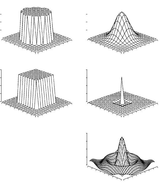
Figure 24-3 shows several common PSFs. In (a), the pillbox has a circular top and straight sides. For example, if the lens of a camera is not properly focused, each point in the image will be projected to a circular spot on the image sensor (look back at Fig. 23-2 and consider the effect of moving the projection screen toward or away from the lens). In other words, the pillbox is the point spread function of an out-of-focus lens.

The Gaussian, shown in (b), is the PSF of imaging systems limited by random imperfections. For instance, the image from a telescope is blurred by atmospheric turbulence, causing each point of light to become a Gaussian in the final image. Image sensors, such as the CCD and retina, are often limited by the scattering of light and/or electrons. The Central Limit Theorem dictates that a Gaussian blur results from these types of random processes.

The pillbox and Gaussian are used in image processing the same as the moving average filter is used with one-dimensional signals. An image convolved with these PSFs will appear blurry and have less defined edges, but will be lower in random noise. These are called smoothing filters, for their action in the time domain, or low-pass filters, for how they treat the frequency domain. The square PSF, shown in (c), can also be used as a smoothing filter, but it is not circularly symmetric. This results in the blurring being different in the diagonal directions compared to the vertical and horizontal. This may or may not be important, depending on the use.

The opposite of a smoothing filter is an edge enhancement or high-pass filter. The spectral inversion technique, discussed in Chapter 14, is used to change between the two. As illustrated in (d), an edge enhancement filter kernel is formed by taking the negative of a smoothing filter, and adding a delta function in the center. The image processing which occurs in the retina is an example of this type of filter.

Figure (e) shows the two-dimensional sinc function. One-dimensional signal processing uses the windowed-sinc to separate frequency bands. Since images do not have their information encoded in the frequency domain, the sinc function is seldom used as an imaging filter kernel, although it does find use in some theoretical problems. The sinc function can be hard to use because its tails decrease very slowly in amplitude ( 1/x ), meaning it must be treated as infinitely wide. In comparison, the Gaussian's tails decrease very rapidly ( e &x 2 ) and can eventually be truncated with no ill effect.

value

4

3

2

1

0

			Chapter 24Linear Image Processing										401
	a. Pillbox							b. Gaussian
						4
						3
						value
						2
						1
						0
-8					8	-8							8
-6						-6
					6								6
-4					4	-4							4
-2					2	-2							2
0		2		-2	0	0			2			-2	0
	row		-4		col			row		4	-4		col
		4
		6	-6							6	-6
		8	-8							8	-8

value

c. Square

4

3

2

1

0

	-8				8
	-6
					6
	-4				4
	-2				2
	0	2		-2	0
	row		-4		col
		4
		6	-6
		8	-8

value

d. Edge enhancement

4

3

2

1

0

	-8				8
	-6
					6
	-4				4
	-2				2
	0	2		-2	0
	row		-4		col
		4
		6	-6
		8	-8

FIGURE 24-3

Common point spread functions. The pillbox, Gaussian, and square, shown in (a), (b), & (c), are common smoothing (low-pass) filters. Edge enhancement (high-pass) filters are formed by subtracting a low-pass kernel from an impulse, as shown in (d). The sinc function, (e), is used very little in image processing because images have their information encoded in the spatial domain, not the frequency domain.

value

e. Sinc

4

3

2

1

0

	-8				8
	-6
					6
	-4				4
	-2				2
	0	2		-2	0
	row		-4		col
		4
		6	-6
		8	-8

All these filter kernels use negative indexes in the rows and columns, allowing the PSF to be centered at row = 0 and column = 0. Negative indexes are often eliminated in one-dimensional DSP by shifting the filter kernel to the right until all the nonzero samples have a positive index. This shift moves the output signal by an equal amount, which is usually of no concern. In comparison, a shift between the input and output images is generally not acceptable. Correspondingly, negative indexes are the norm for filter kernels in image processing.