TsOS / DSP_guide_Smith / Ch15

CHAPTER

Moving Average Filters

15

The moving average is the most common filter in DSP, mainly because it is the easiest digital filter to understand and use. In spite of its simplicity, the moving average filter is optimal for a common task: reducing random noise while retaining a sharp step response. This makes it the premier filter for time domain encoded signals. However, the moving average is the worst filter for frequency domain encoded signals, with little ability to separate one band of frequencies from another. Relatives of the moving average filter include the Gaussian, Blackman, and multiplepass moving average. These have slightly better performance in the frequency domain, at the expense of increased computation time.

Implementation by Convolution

As the name implies, the moving average filter operates by averaging a number of points from the input signal to produce each point in the output signal. In equation form, this is written:

EQUATION 15-1

Equation of the moving average filter. In this equation, x[ ] is the input signal, y[ ] is the output signal, and M is the number of points used in the moving average. This equation only uses points on one side of the output sample being calculated.

		1	M & 1
	y [i ] '		j x [ i % j ]
		M
			j' 0

Where x [ ] is the input signal, y [ ] is the output signal, and M is the number of points in the average. For example, in a 5 point moving average filter, point 80 in the output signal is given by:

y [80] ' x [80] % x [81] % x [82] % x [83] % x [84] 5

277

278	The Scientist and Engineer's Guide to Digital Signal Processing

As an alternative, the group of points from the input signal can be chosen symmetrically around the output point:

y [80] ' x [78] % x [79] % x [80] % x [81] % x [82] 5

This corresponds to changing the summation in Eq. 15-1 from: j ' 0 to M& 1 , to: j ' & (M& 1) /2 to (M& 1) /2 . For instance, in an 11 point moving average filter, the index, j, can run from 0 to 11 (one side averaging) or -5 to 5 (symmetrical averaging). Symmetrical averaging requires that M be an odd number. Programming is slightly easier with the points on only one side; however, this produces a relative shift between the input and output signals.

You should recognize that the moving average filter is a convolution using a very simple filter kernel. For example, a 5 point filter has the filter kernel: þ 0, 0, 1/5, 1/5, 1/5, 1/5, 1/5, 0, 0 þ . That is, the moving average filter is a convolution of the input signal with a rectangular pulse having an area of one. Table 15-1 shows a program to implement the moving average filter.

100 'MOVING AVERAGE FILTER

110 'This program filters 5000 samples with a 101 point moving 120 'average filter, resulting in 4900 samples of filtered data. 130 '

140	DIM X[4999]	'X[ ] holds the input signal
150	DIM Y[4999]	'Y[ ] holds the output signal
160 '
170	GOSUB XXXX	'Mythical subroutine to load X[ ]
180 '
190 FOR I% = 50 TO 4949		'Loop for each point in the output signal
200	Y[I%] = 0	'Zero, so it can be used as an accumulator
210	FOR J% = -50 TO 50	'Calculate the summation
220	Y[I%] = Y[I%] + X(I%+J%]
230	NEXT J%
240	Y[I%] = Y[I%]/101	'Complete the average by dividing

250 NEXT I%

260 '

270 END

TABLE 15-1

Noise Reduction vs. Step Response

Many scientists and engineers feel guilty about using the moving average filter. Because it is so very simple, the moving average filter is often the first thing tried when faced with a problem. Even if the problem is completely solved, there is still the feeling that something more should be done. This situation is truly ironic. Not only is the moving average filter very good for many applications, it is optimal for a common problem, reducing random white noise while keeping the sharpest step response.

Chapter 15Moving Average Filters

279

2
a.	Original signal
1
Amplitude
0
-1
0	100	200	300	400	500

Sample number

2
	b. 11 point moving average
1
Amplitude
0
-1
0	100	200	300	400	500

Sample number

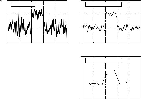
FIGURE 15-1

Example of a moving average filter. In (a), a rectangular pulse is buried in random noise. In

(b) and (c), this signal is filtered with 11 and 51 point moving average filters, respectively. As the number of points in the filter increases, the noise becomes lower; however, the edges becoming less sharp. The moving average filter is the optimal solution for this problem, providing the lowest noise possible for a given edge sharpness.

Amplitude

2

c. 51 point moving average

1

0

-1

0

100

200

300

400

500

Sample number

Figure 15-1 shows an example of how this works. The signal in (a) is a pulse buried in random noise. In (b) and (c), the smoothing action of the moving average filter decreases the amplitude of the random noise (good), but also reduces the sharpness of the edges (bad). Of all the possible linear filters that could be used, the moving average produces the lowest noise for a given edge sharpness. The amount of noise reduction is equal to the square-root of the number of points in the average. For example, a 100 point moving average filter reduces the noise by a factor of 10.

To understand why the moving average if the best solution, imagine we want to design a filter with a fixed edge sharpness. For example, let's assume we fix the edge sharpness by specifying that there are eleven points in the rise of the step response. This requires that the filter kernel have eleven points. The optimization question is: how do we choose the eleven values in the filter kernel to minimize the noise on the output signal? Since the noise we are trying to reduce is random, none of the input points is special; each is just as noisy as its neighbor. Therefore, it is useless to give preferential treatment to any one of the input points by assigning it a larger coefficient in the filter kernel. The lowest noise is obtained when all the input samples are treated equally, i.e., the moving average filter. (Later in this chapter we show that other filters are essentially as good. The point is, no filter is better than the simple moving average).

280	The Scientist and Engineer's Guide to Digital Signal Processing

Frequency Response

Figure 15-2 shows the frequency response of the moving average filter. It is mathematically described by the Fourier transform of the rectangular pulse, as discussed in Chapter 11:

EQUATION 15-2

Frequency response of an M point moving average filter. The frequency, f, runs between 0 and 0.5. For f ' 0 , use: H [ f ] ' 1

H [ f ] ' sin(Bf M ) M sin(Bf )

The roll-off is very slow and the stopband attenuation is ghastly. Clearly, the moving average filter cannot separate one band of frequencies from another. Remember, good performance in the time domain results in poor performance in the frequency domain, and vice versa. In short, the moving average is an exceptionally good smoothing filter (the action in the time domain), but an exceptionally bad low-pass filter (the action in the frequency domain).

FIGURE 15-2

Frequency response of the moving average filter. The moving average is a very poor low-pass filter, due to its slow roll-off and poor stopband attenuation. These curves are generated by Eq. 15-2.

	1.2
	1.0
		3 point
Amplitude	0.8
	0.6	11 point
	0.4	31 point
	0.2
	0.0
	0	0.1	0.2	0.3	0.4	0.5
			Frequency

Relatives of the Moving Average Filter

In a perfect world, filter designers would only have to deal with time domain or frequency domain encoded information, but never a mixture of the two in the same signal. Unfortunately, there are some applications where both domains are simultaneously important. For instance, television signals fall into this nasty category. Video information is encoded in the time domain, that is, the shape of the waveform corresponds to the patterns of brightness in the image. However, during transmission the video signal is treated according to its frequency composition, such as its total bandwidth, how the carrier waves for sound & color are added, elimination & restoration of the DC component, etc. As another example, electromagnetic interference is best understood in the frequency domain, even if

Chapter 15Moving Average Filters

281

Amplitude

Amplitude

0.2			1.25
a. Filter kernel				c. Frequency response
	1 pass		1.00
2 pass	FFT	Amplitude	0.75	1 pass
0.1				2 pass
			0.50
				4 pass
	4 pass		0.25

0.0					0.00
0	6	12	18	24	0	0.1	0.2	0.3	0.4	0.5
		Sample number					Frequency
		Integrate					20 Log(		)
1.2					40
	b. Step response				20	d. Frequency response (dB)
1.0
0.8		1 pass	4 pass	(dB)	0		1 pass
					-20
0.6				Amplitude	-40
0.4					-60
					-80	2 pass
0.2					-100	4 pass
		2 pass
0.0					-120
0	6	12	18	24	0	0.1	0.2	0.3	0.4	0.5
		Sample number					Frequency

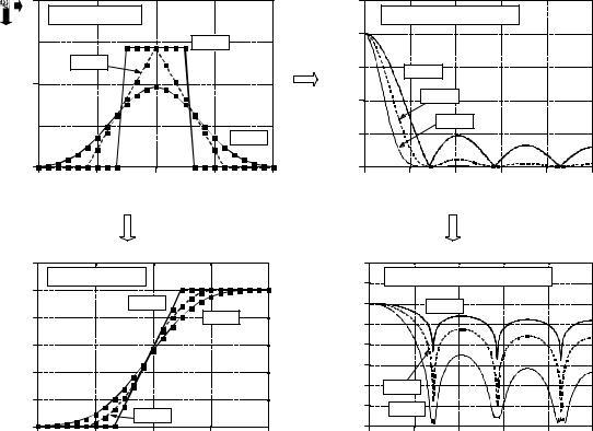
FIGURE 15-3

Characteristics of multiple-pass moving average filters. Figure (a) shows the filter kernels resulting from passing a seven point moving average filter over the data once, twice and four times. Figure (b) shows the corresponding step responses, while (c) and (d) show the corresponding frequency responses.

the signal's information is encoded in the time domain. For instance, the temperature monitor in a scientific experiment might be contaminated with 60 hertz from the power lines, 30 kHz from a switching power supply, or 1320 kHz from a local AM radio station. Relatives of the moving average filter have better frequency domain performance, and can be useful in these mixed domain applications.

Multiple-pass moving average filters involve passing the input signal through a moving average filter two or more times. Figure 15-3a shows the overall filter kernel resulting from one, two and four passes. Two passes are equivalent to using a triangular filter kernel (a rectangular filter kernel convolved with itself). After four or more passes, the equivalent filter kernel looks like a Gaussian (recall the Central Limit Theorem). As shown in (b), multiple passes produce an "s" shaped step response, as compared to the straight line of the single pass. The frequency responses in (c) and (d) are given by Eq. 15-2 multiplied by itself for each pass. That is, each time domain convolution results in a multiplication of the frequency spectra.

282	The Scientist and Engineer's Guide to Digital Signal Processing

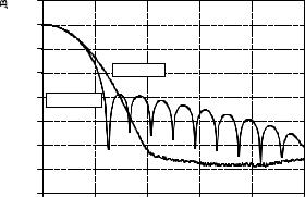
Figure 15-4 shows the frequency response of two other relatives of the moving average filter. When a pure Gaussian is used as a filter kernel, the frequency response is also a Gaussian, as discussed in Chapter 11. The Gaussian is important because it is the impulse response of many natural and manmade systems. For example, a brief pulse of light entering a long fiber optic transmission line will exit as a Gaussian pulse, due to the different paths taken by the photons within the fiber. The Gaussian filter kernel is also used extensively in image processing because it has unique properties that allow fast two-dimensional convolutions (see Chapter 24). The second frequency response in Fig. 15-4 corresponds to using a Blackman window as a filter kernel. (The term window has no meaning here; it is simply part of the accepted name of this curve). The exact shape of the Blackman window is given in Chapter 16 (Eq. 16-2, Fig. 16-2); however, it looks much like a Gaussian.

How are these relatives of the moving average filter better than the moving average filter itself? Three ways: First, and most important, these filters have better stopband attenuation than the moving average filter. Second, the filter kernels taper to a smaller amplitude near the ends. Recall that each point in the output signal is a weighted sum of a group of samples from the input. If the filter kernel tapers, samples in the input signal that are farther away are given less weight than those close by. Third, the step responses are smooth curves, rather than the abrupt straight line of the moving average. These last two are usually of limited benefit, although you might find applications where they are genuine advantages.

The moving average filter and its relatives are all about the same at reducing random noise while maintaining a sharp step response. The ambiguity lies in how the risetime of the step response is measured. If the risetime is measured from 0% to 100% of the step, the moving average filter is the best you can do, as previously shown. In comparison, measuring the risetime from 10% to 90% makes the Blackman window better than the moving average filter. The point is, this is just theoretical squabbling; consider these filters equal in this parameter.

The biggest difference in these filters is execution speed. Using a recursive algorithm (described next), the moving average filter will run like lightning in your computer. In fact, it is the fastest digital filter available. Multiple passes of the moving average will be correspondingly slower, but still very quick. In comparison, the Gaussian and Blackman filters are excruciatingly slow, because they must use convolution. Think a factor of ten times the number of points in the filter kernel (based on multiplication being about 10 times slower than addition). For example, expect a 100 point Gaussian to be 1000 times slower than a moving average using recursion.

Recursive Implementation

A tremendous advantage of the moving average filter is that it can be implemented with an algorithm that is very fast. To understand this

Chapter 15Moving Average Filters

283

FIGURE 15-4

Frequency response of the Blackman window and Gaussian filter kernels. Both these filters provide better stopband attenuation than the moving average filter. This has no advantage in removing random noise from time domain encoded signals, but it can be useful in mixed domain problems. The disadvantage of these filters is that they must use convolution, a terribly slow algorithm.

	20
	0
	-20
(dB)	-40		Gaussian
Amplitude	-60	Blackman
	-80
	-100
	-120
	-140
	0	0.1	0.2	0.3	0.4	0.5
			Frequency

algorithm, imagine passing an input signal, x [ ], through a seven point moving average filter to form an output signal, y [ ]. Now look at how two adjacent output points, y [50] and y [51], are calculated:

y [50] ' x [47] % x [48] % x [49] % x [50] % x [51] % x [52] % x [53]

y [51] ' x [48] % x [49] % x [50] % x [51] % x [52] % x [53] % x [54]

These are nearly the same calculation; points x [48] through x [53] must be added for y [50], and again for y [51]. If y [50] has already been calculated, the most efficient way to calculate y [51] is:

y [51] ' y [50] % x [54] & x [47]

Once y [51] has been found using y [50], then y [52] can be calculated from sample y [51], and so on. After the first point is calculated in y [ ], all of the other points can be found with only a single addition and subtraction per point. This can be expressed in the equation:

	EQUATION 15-3
	Recursive implementation of the moving	y [i ] ' y [i & 1] % x [i % p ] & x [i & q ]
	average filter. In this equation, x[ ] is the
	input signal, y[ ] is the output signal, M is the
	number of points in the moving average (an	where:	p ' (M& 1) /2
	odd number). Before this equation can be
	used, the first point in the signal must be		q ' p % 1
	calculated using a standard summation.

Notice that this equation use two sources of data to calculate each point in the output: points from the input and previously calculated points from the output. This is called a recursive equation, meaning that the result of one calculation

284	The Scientist and Engineer's Guide to Digital Signal Processing
	is used in future calculations. (The term "recursive" also has other meanings,
	especially in computer science). Chapter 19 discusses a variety of recursive
	filters in more detail. Be aware that the moving average recursive filter is very
	different from typical recursive filters. In particular, most recursive filters have
	an infinitely long impulse response (IIR), composed of sinusoids and
	exponentials. The impulse response of the moving average is a rectangular
	pulse (finite impulse response, or FIR).
	This algorithm is faster than other digital filters for several reasons. First,
	there are only two computations per point, regardless of the length of the filter
	kernel. Second, addition and subtraction are the only math operations needed,
	while most digital filters require time-consuming multiplication. Third, the
	indexing scheme is very simple. Each index in Eq. 15-3 is found by adding or
	subtracting integer constants that can be calculated before the filtering starts
	(i.e., p and q). Forth, the entire algorithm can be carried out with integer
	representation. Depending on the hardware used, integers can be more than an
	order of magnitude faster than floating point.
	Surprisingly, integer representation works better than floating point with this
	algorithm, in addition to being faster. The round-off error from floating point
	arithmetic can produce unexpected results if you are not careful. For example,
	imagine a 10,000 sample signal being filtered with this method. The last
	sample in the filtered signal contains the accumulated error of 10,000 additions
	and 10,000 subtractions. This appears in the output signal as a drifting offset.
	Integers don't have this problem because there is no round-off error in the
	arithmetic. If you must use floating point with this algorithm, the program in
	Table 15-2 shows how to use a double precision accumulator to eliminate this
	drift.
100	'MOVING AVERAGE FILTER IMPLEMENTED BY RECURSION
110	'This program filters 5000 samples with a 101 point moving
120 'average filter, resulting in 4900 samples of filtered data.
130	'A double precision accumulator is used to prevent round-off drift.
140	'
150	DIM X[4999]	'X[ ] holds the input signal
160	DIM Y[4999]	'Y[ ] holds the output signal
170	DEFDBL ACC	'Define the variable ACC to be double precision
180	'
190	GOSUB XXXX	'Mythical subroutine to load X[ ]
200	'
210	ACC = 0	'Find Y[50] by averaging points X[0] to X[100]
220 FOR I% = 0 TO 100
230	ACC = ACC + X[I%]
240 NEXT I%
250	Y[[50] = ACC/101
260	'	'Recursive moving average filter (Eq. 15-3)
270 FOR I% = 51 TO 4949
280	ACC = ACC + X[I%+50] - X[I%-51]
290	Y[I%] = ACC
300 NEXT I%
310	'
320 END		TABLE 15-2