TsOS / DSP_guide_Smith / Ch18

CHAPTER

FFT Convolution

18

This chapter presents two important DSP techniques, the overlap-add method, and FFT convolution. The overlap-add method is used to break long signals into smaller segments for easier processing. FFT convolution uses the overlap-add method together with the Fast Fourier Transform, allowing signals to be convolved by multiplying their frequency spectra. For filter kernels longer than about 64 points, FFT convolution is faster than standard convolution, while producing exactly the same result.

The Overlap-Add Method

There are many DSP applications where a long signal must be filtered in segments. For instance, high fidelity digital audio requires a data rate of about 5 Mbytes/min, while digital video requires about 500 Mbytes/min. With data rates this high, it is common for computers to have insufficient memory to simultaneously hold the entire signal to be processed. There are also systems that process segment-by-segment because they operate in real time. For example, telephone signals cannot be delayed by more than a few hundred milliseconds, limiting the amount of data that are available for processing at any one instant. In still other applications, the processing may require that the signal be segmented. An example is FFT convolution, the main topic of this chapter.

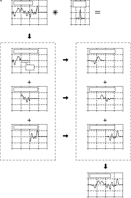
The overlap-add method is based on the fundamental technique in DSP: (1) decompose the signal into simple components, (2) process each of the components in some useful way, and (3) recombine the processed components into the final signal. Figure 18-1 shows an example of how this is done for the overlap-add method. Figure (a) is the signal to be filtered, while (b) shows the filter kernel to be used, a windowed-sinc low-pass filter. Jumping to the bottom of the figure, (i) shows the filtered signal, a smoothed version of (a). The key to this method is how the lengths of these signals are affected by the convolution. When an N sample signal is convolved with an M sample

311

312	The Scientist and Engineer's Guide to Digital Signal Processing

filter kernel, the output signal is N% M& 1 samples long. For instance, the input signal, (a), is 300 samples (running from 0 to 299), the filter kernel, (b), is 101 samples (running from 0 to 100), and the output signal, (i), is 400 samples (running from 0 to 399).

In other words, when an N sample signal is filtered, it will be expanded by M& 1 points to the right. (This is assuming that the filter kernel runs from index 0 to M. If negative indexes are used in the filter kernel, the expansion will also be to the left). In (a), zeros have been added to the signal between sample 300 and 399 to illustrate where this expansion will occur. Don't be confused by the small values at the ends of the output signal, (i). This is simply a result of the windowed-sinc filter kernel having small values near its ends. All 400 samples in (i) are nonzero, even though some of them are too small to be seen in the graph.

Figures (c), (d) and (e) show the decomposition used in the overlap-add method. The signal is broken into segments, with each segment having 100 samples from the original signal. In addition, 100 zeros are added to the right of each segment. In the next step, each segment is individually filtered by convolving it with the filter kernel. This produces the output segments shown in (f), (g), and (h). Since each input segment is 100 samples long, and the filter kernel is 101 samples long, each output segment will be 200 samples long. The important point to understand is that the 100 zeros were added to each input segment to allow for the expansion during the convolution.

Notice that the expansion results in the output segments overlapping each other. These overlapping output segments are added to give the output signal, (i). For instance, samples 200 to 299 in (i) are found by adding the corresponding samples in (g) and (h). The overlap-add method produces exactly the same output signal as direct convolution. The disadvantage is a much greater program complexity to keep track of the overlapping samples.

FFT Convolution

FFT convolution uses the principle that multiplication in the frequency domain corresponds to convolution in the time domain. The input signal is transformed into the frequency domain using the DFT, multiplied by the frequency response of the filter, and then transformed back into the time domain using the Inverse DFT. This basic technique was known since the days of Fourier; however, no one really cared. This is because the time required to calculate the DFT was longer than the time to directly calculate the convolution. This changed in 1965 with the development of the Fast Fourier Transform (FFT). By using the FFT algorithm to calculate the DFT, convolution via the frequency domain can be faster than directly convolving the time domain signals. The final result is the same; only the number of calculations has been changed by a more efficient algorithm. For this reason, FFT convolution is also called high-speed convolution.

Chapter 18FFT Convolution

313

	4
		a. Input signal
Amplitude	2
	0
	-2
	-4
	0	100	200	300	400

Sample number

	4
		c. Input segment 1
Amplitude	2
	0
	-2		added
			zeros
	-4
	0	100	200	300	400

	0.180
		b. Filter			?
Amplitude	0.120		kernel
	0.060
	0.000
	-0.060
	-50	0	50	100	150
			Sample

	4
		f. Output segment 1
Amplitude	2
	0
	-2
	-4
	0	100	200	300	400

		Sample number
	4
		d. Input segment 2
Amplitude	2
	0
	-2
	-4
	0	100	200	300	400

		Sample number
	4
		g. Output segment 2
Amplitude	2
	0
	-2
	-4
	0	100	200	300	400

		Sample number
	4
		e. Input segment 3
Amplitude	2
	0
	-2
	-4
	0	100	200	300	400

Sample number

	4
		h. Output segment 3
Amplitude	2
	0
	-2
	-4
	0	100	200	300	400

Sample number

FIGURE 18-1

The overlap-add method. The goal is to convolve the input signal, (a), with the filter kernel, (b). This is done by breaking the input signal into a number of segments, such as (c), (d) and (e), each padded with enough zeros to allow for the expansion during the convolution. Convolving each of the input segments with the filter kernel produces the output segments, (f), (g), and (h). The output signal, (i), is then found by adding the overlapping output segments.

Sample number

	4
		i. Output signal
Amplitude	2
	0
	-2
	-4
	0	100	200	300	400

Sample number

314	The Scientist and Engineer's Guide to Digital Signal Processing

FFT convolution uses the overlap-add method shown in Fig. 18-1; only the way that the input segments are converted into the output segments is changed. Figure 18-2 shows an example of how an input segment is converted into an output segment by FFT convolution. To start, the frequency response of the filter is found by taking the DFT of the filter kernel, using the FFT. For instance, (a) shows an example filter kernel, a windowed-sinc band-pass filter. The FFT converts this into the real and imaginary parts of the frequency response, shown in (b) & (c). These frequency domain signals may not look like a band-pass filter because they are in rectangular form. Remember, polar form is usually best for humans to understand the frequency domain, while rectangular form is normally best for mathematical calculations. These real and imaginary parts are stored in the computer for use when each segment is being calculated.

Figure (d) shows the input segment to being processed. The FFT is used to find its frequency spectrum, shown in (e) & (f). The frequency spectrum of the output segment, (h) & (i) is then found by multiplying the filter's frequency response, (b) & (c), by the spectrum of the input segment, (e) & (f). Since these spectra consist of real and imaginary parts, they are multiplied according to Eq. 9-1 in Chapter 9. The Inverse FFT is then used to find the output segment, (g), from its frequency spectrum, (h) & (i). It is important to recognize that this output segment is exactly the same as would be obtained by the direct convolution of the input segment, (d), and the filter kernel, (a).

The FFTs must be long enough that circular convolution does not take place (also described in Chapter 9). This means that the FFT should be the same length as the output segment, (g). For instance, in the example of Fig. 18-2, the filter kernel contains 129 points and each segment contains 128 points, making output segment 256 points long. This calls for 256 point FFTs to be used. This means that the filter kernel, (a), must be padded with 127 zeros to bring it to a total length of 256 points. Likewise, each of the input segments, (d), must be padded with 128 zeros. As another example, imagine you need to convolve a very long signal with a filter kernel having 600 samples. One alternative would be to use segments of 425 points, and 1024 point FFTs. Another alternative would be to use segments of 1449 points, and 2048 point FFTs.

Table 18-1 shows an example program to carry out FFT convolution. This program filters a 10 million point signal by convolving it with a 400 point filter kernel. This is done by breaking the input signal into 16000 segments, with each segment having 625 points. When each of these segments is convolved with the filter kernel, an output segment of 625 % 400 & 1 ' 1024 points is produced. Thus, 1024 point FFTs are used. After defining and initializing all the arrays (lines 130 to 230), the first step is to calculate and store the frequency response of the filter (lines 250 to 310). Line 260 calls a mythical subroutine that loads the filter kernel into XX[0] through XX[399], and sets XX[400] through XX[1023] to a value of zero. The subroutine in line 270 is the FFT, transforming the 1024 samples held in XX[ ] into the 513 samples held in REX[ ] & IMX[ ], the real and

	Chapter 18FFT Convolution	315
Time Domain	Frequency Domain

	0.3						2.0					2.0
	0.2	a. Filter kernel							b. Real				c. Imaginary
							1.0					1.0
Amplitude						Amplitude					Amplitude
	0.1				FFT
							0.0					0.0
	0.0
	-0.1		signal in 0 to 128				-1.0					-1.0
			zeros in 129 to 255
	-0.2						-2.0					-2.0
	0	64	128	192	2565			0	64	128		0	64	128
		Sample number							Frequency				Frequency
	6.0						100					100
	4.0	d. Input segment							e. Real				f. Imaginary
							50					50
Amplitude	2.0				FFT	Amplitude					Amplitude
	0.0						0					0
	-2.0
							-50					-50

-4.0						signal in 0 to 127
						zeros in 128 to 255
-6.0														-100							-100
0			64			128			192			2565		0		64			128		0		64			128
					Sample number											Frequency							Frequency

	6.0							100					100
	4.0	g.	Output segment							h. Real				i. Imaginary
								50					50
Amplitude	2.0					IFFT	Amplitude					Amplitude
	0.0							0					0
	-2.0
								-50					-50
	-4.0			signal in 0 to 255
	-6.0							-100					-100
	0		64	128	192	2565			0	64	128		0	64	128
			Sample number							Frequency				Frequency

FIGURE 18-2

FFT convolution. The filter kernel, (a), and the signal segment, (d), are converted into their respective spectra,

(b) & (c) and (d) & (e), via the FFT. These spectra are multiplied, resulting in the spectrum of the output segment, (h) & (i). The Inverse FFT then finds the output segment, (g).

imaginary parts of the frequency response. These values are transferred into the arrays REFR[ ] & IMFR[ ] (for: REal and IMaginary Frequency Response), to be used later in the program.

316	The Scientist and Engineer's Guide to Digital Signal Processing

The FOR-NEXT loop between lines 340 and 580 controls how the 16000 segments are processed. In line 360, a subroutine loads the next segment to be processed into XX[0] through XX[624], and sets XX[625] through XX[1023] to a value of zero. In line 370, the FFT subroutine is used to find this segment's frequency spectrum, with the real part being placed in the 513 points of REX[ ], and the imaginary part being placed in the 513 points of IMX[ ]. Lines 390 to 430 show the multiplication of the segment's frequency spectrum, held in REX[ ] & IMX[ ], by the filter's frequency response, held in REFR[ ] and IMFR[ ]. The result of the multiplication is stored in REX[ ] & IMX[ ], overwriting the data previously there. Since this is now the frequency spectrum of the output segment, the IFFT can be used to find the output segment. This is done by the mythical IFFT subroutine in line 450, which transforms the 513 points held in REX[ ] & IMX[ ] into the 1024 points held in XX[ ], the output segment.

Lines 470 to 550 handle the overlapping of the segments. Each output segment is divided into two sections. The first 625 points (0 to 624) need to be combined with the overlap from the previous output segment, and then written to the output signal. The last 399 points (625 to 1023) need to be saved so that they can overlap with the next output segment.

To understand this, look back at Fig 18-1. Samples 100 to 199 in (g) need to be combined with the overlap from the previous output segment, (f), and can then be moved to the output signal (i). In comparison, samples 200 to 299 in

(g) need to be saved so that they can be combined with the next output segment, (h).

Now back to the program. The array OLAP[ ] is used to hold the 399 samples that overlap from one segment to the next. In lines 470 to 490 the 399 values in this array (from the previous output segment) are added to the output segment currently being worked on, held in XX[ ]. The mythical subroutine in line 550 then outputs the 625 samples in XX[0] to XX[624] to the file holding the output signal. The 399 samples of the current output segment that need to be held over to the next output segment are then stored in OLAP[ ] in lines 510 to 530.

After all 0 to 15999 segments have been processed, the array, OLAP[ ], will contain the 399 samples from segment 15999 that should overlap segment 16000. Since segment 16000 doesn't exist (or can be viewed as containing all zeros), the 399 samples are written to the output signal in line 600. This makes the length of the output signal 16000 × 625 % 399 ' 10,000,399 points. This matches the length of input signal, plus the length of the filter kernel, minus 1.

Speed Improvements

When is FFT convolution faster than standard convolution? The answer depends on the length of the filter kernel, as shown in Fig. 18-3. The time

			Chapter 18FFT Convolution	317
100	'FFT CONVOLUTION
110	'This program convolves a 10 million point signal with a 400 point filter kernel. The input
120	'signal is broken into 16000 segments, each with 625 points. 1024 point FFTs are used.
130	'
130	'		'INITIALIZE THE ARRAYS
140	DIM XX[1023]		'the time domain signal (for the FFT)
150	DIM REX[512]		'real part of the frequency domain (for the FFT)
160	DIM IMX[512]		'imaginary part of the frequency domain (for the FFT)
170	DIM REFR[512]		'real part of the filter's frequency response
180	DIM IMFR[512]		'imaginary part of the filter's frequency response
190	DIM OLAP[398]		'holds the overlapping samples from segment to segment
200	'
210	FOR I% = 0 TO 398		'zero the array holding the overlapping samples
220	OLAP[I%] = 0
230 NEXT I%
240	'
250	'		'FIND & STORE THE FILTER'S FREQUENCY RESPONSE
260	GOSUB XXXX		'Mythical subroutine to load the filter kernel into XX[ ]
270	GOSUB XXXX		'Mythical FFT subroutine: XX[ ] --> REX[ ] & IMX[ ]
280	FOR F% = 0 TO 512		'Save the frequency response in REFR[ ] & IMFR[ ]
290	REFR[F%] = REX[F%]
300	IMFR[F%] = IMX[F%]
310 NEXT F%
320	'
330	'		'PROCESS EACH OF THE 16000 SEGMENTS
340 FOR SEGMENT% = 0 TO 15999
350	'
360	GOSUB XXXX		'Mythical subroutine to load the next input segment into XX[ ]
370	GOSUB XXXX		'Mythical FFT subroutine: XX[ ] --> REX[ ] & IMX[ ]
380	'
390	FOR F% = 0 TO 512 'Multiply the frequency spectrum by the frequency response
400	TEMP	= REX[F%]*REFR[F%] - IMX[F%]*IMFR[F%]
410	IMX[F%]	= REX[F%]*IMFR[F%] + IMX[F%]*REFR[F%]
420	REX[F%]	= TEMP
430	NEXT F%
440	'
450	GOSUB XXXX		'Mythical IFFT subroutine: REX[ ] & IMX[ ] --> XX[ ]
460	'
470	FOR I% = 0 TO 398 'Add the last segment's overlap to this segment
480	XX[I%] = XX[I%] + OLAP[I%]
490	NEXT I%
500	'
510	FOR I% = 625 TO 1023		'Save the samples that will overlap the next segment
520	OLAP[I%-625] = XX[I%]
530	NEXT I%
540	'
550	GOSUB XXXX		'Mythical subroutine to output the 625 samples stored
560	'		'in XX[0] to XX[624]
570	'
580 NEXT SEGMENT%
590	'
600	GOSUB XXXX		'Mythical subroutine to output all 399 samples in OLAP[ ]

610 END

TABLE 18-1

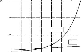
for standard convolution is directly proportional to the number of points in the filter kernel. In comparison, the time required for FFT convolution increases very slowly, only as the logarithm of the number of points in the

318	The Scientist and Engineer's Guide to Digital Signal Processing

FIGURE 18-3

Execution times for FFT convolution. FFT convolution is faster than the standard method when the filter kernel is longer than about 60 points. These execution times are for a 100 MHz Pentium, using single precision floating point.

(msec/point)Time	1.5
	1					Standard
Execution	0.5
								FFT
	0	8	16	32	64	128	256	512	1024

Impulse Response Length

filter kernel. The crossover occurs when the filter kernel has about 40 to 80 samples (depending on the particular hardware used).

The important idea to remember: filter kernels shorter than about 60 points can be implemented faster with standard convolution, and the execution time is proportional to the kernel length. Longer filter kernels can be implemented faster with FFT convolution. With FFT convolution, the filter kernel can be made as long as you like, with very little penalty in execution time. For instance, a 16,000 point filter kernel only requires about twice as long to execute as one with only 64 points.

The speed of the convolution also dictates the precision of the calculation (just as described for the FFT in Chapter 12). This is because the round-off error in the output signal depends on the total number of calculations, which is directly proportional to the computation time. If the output signal is calculated faster, it will also be calculated more precisely. For instance, imagine convolving a signal with a 1000 point filter kernel, with single precision floating point. Using standard convolution, the typical round-off noise can be expected to be about 1 part in 20,000 (from the guidelines in Chapter 4). In comparison, FFT convolution can be expected to be an order of magnitude faster, and an order of magnitude more precise (i.e., 1 part in 200,000).

Keep FFT convolution tucked away for when you have a large amount of data to process and need an extremely long filter kernel. Think in terms of a million sample signal and a thousand point filter kernel. Anything less won't justify the extra programming effort. Don't want to write your own FFT convolution routine? Look in software libraries and packages for prewritten code. Start with this book's web site (see the copyright page).