Как получить 8 за 5 дней

Next, let us consider the effect of disutility of effort on the IC constraint: an increase in disutility of effort results in a upward shift in IC for as long as it is smaller than the difference between the probabilities of success in cases of high and low effort ( (1) x(1) x(0) ), thereby, causing some part of IC to exceed the BC line, and thus to violate the BC constraint (see Fig. A4 in appendix). Thus, the higher the disutility of effort (for example the difficulty of task), the higher intrinsic motivation is required from the agent, bonus to be consistent with the BC constraint.

Alternatively, let us consider the case when the disutility of effort exceeds the probability effect of effort ( (1) x(1) x(0) ): in this case the IC curve will have a different shape (see Fig. A5), sloping upwards for higher levels of a, as well as shifting upwards as (1) increases. The different shape, however will not significantly affect the bonus policy, as the actual bonus paid is still decreasing in a. But it ensures all agents with a higher than some critical level (the intersection of IC and BC), will be paid non-zero bonus, except for the case when a=1. Essentially, this difference is not a serious one, as highly motivated agents, will have a very small monetary reward. The essential difference arises, when (1) is significantly higher than x(1) x(0) . In such case the IC will be fully located above the BC (Fig. A6) and the principal will assign a bonus of zero. In the case when the disutility of effort is proportional to the probability effect of effort ( (1) x(1) x(0) ) the IC becomes a linear function (Fig. A7), the implications of which for the equilibrium are the same as the case when (1) is higher.

The factor that affects both constraints is the kind of the function of probability of success relative to the level of effort. In our case, as the situation is binary, only x(1) and x(0) affect the graphs. The factor, affecting the BC constraint, is the difference between probabilities of success in cases of high and low effort relative to the probability of success in case of high effort. If we look thoroughly at (10) we can see that its effect is analogous to the effect of magnitude of ρ: a decrease in this

20

difference shifts the BC down. On the other hand, the CS constraint is also affected by the difference in probabilities. If we look at (9), we can see, that it‟s effect is opposite to the disutility of effort effect: the higher the difference, the lower is the b required to stimulate high effort. Thus, if this difference is smaller the CS curve shifts up. The overall effect of the decrease of the probability effect of effort is obvious: much higher intrinsic motivation would be required from the agent, for it the principle to set an effective bonus (see Fig. A8 and compare with Fig. 2).

3.2.3. Advantages, Drawbacks and Possible Modifications

On the positive side of this game within the model setup, being quite simple, it accounts for multiple factors that may affect contractual relationships, including the psychological component as well. The stylized facts, as derived in the parameter analysis, are consistent with common sense, as well as with claims of economic, sociological and psychological perspectives, concerning motivation. It provides an economic account of intrinsic motivation (a somewhat psychological term), as well as of issues like trust and beliefs.

A disadvantage of such a presentation might be rooted in the model simplicity. Undoubtedly, in the real world an agent is not limited to a binary choice between high and low level of effort, neither is the fixed wage uniform with all principals, so the agent‟s loyalty is a matter of dynamic games with the principal. The model is appropriate for dynamic analysis and will allow to draw yet even more interesting conclusions on the P-A relationships in presence of the moral hazard problem; however, in this work it will not be presented in detail. As far as the level of effort is concerned, complying with the dimensionality of the game above it can be established at any level between 0 and 1 where, 1 would denote some natural capacity that can not be exceeded. The function of probability of success, as a result, will also be continuous, and its form is of particular interest and is individual for each project, though might

21

be quite similar for projects that are alike. The attempt to present a more or less realistic shape of x(e) is provided in appendix (Fig. A9). At low levels of effort marginal probability may increase for lower levels of effort, while fall at higher effort levels.

The disutility of effort is also expected to be a continuous function, the form of which is also extremely important, and is hard to estimate, as it is a psychological component. In fact it is possible that (1) (0) , if, for instance, for a self-disciplined agent it is even worse to “loaf around” at the workplace, than to do some work. In general, the disutility of effort is an individual characteristic and can take any imaginable form, depending on an agent‟s personality. This issue is also hard to account for as, disutility of effort is hard to quantify and in fact the agent, himself, may be unaware of its magnitude.

The beliefs may enter the payoff functions of the actors in a much more complicated way in reality, and are also hard to observe. In fact, the beliefs may concern other variables. Strictly speaking, the game presented above is not a psychological game as defined by Geanakoplos Pierce Stacchetti [2], though it does include a psychological component (beliefs). The authors define a psychological game as a game where the payoffs depend on multilevel beliefs about the counteragent‟s set of strategies, while the game above includes beliefs about some property of project, rather than the strategy of the agent. Moreover, this property was treated as exogenous in the game presented. However, this flaw can be settled, through minor game modifications. Below some of such variations are given.

3.2.3.1. Endogenizing Theta

Let us attempt to redefine as an endogenous variable. Technically the easiest way to do this, is to claim that is chosen by the agent, as an intrinsic attitude to the project work. The form of the game will not change, and it will be good for the agent to set high if he believes, that he is expected to value the success of the project highly, and

22

as this belief weakens, the reward value m , falls as the marginal effect of , thus resulting in a lower and causing the crowding out of the intrinsic motivation by extrinsic, as the expected bonus 1 m b grows. This, however, is a minor change and still does not make the game a “proper” psychological game.

3.2.3.2. A Principal’s Perspective Game

In this game we assume, that the level of can be affected by the principal‟s HR policy. This game is more relevant to the case of office jobs, where is initially low, while the previous game allowed to consider cases with different initial ‟s. Now in an industry with low , the HR policy allows to increase . For the sake of this game, let us assume is zero in case of no policy, and positive in case if policy is taken. However, the policy requires a sunk cost of conduction to commit by the principal, as when approved the HR policy can not be reversed.

Let us introduce an additional variable and redefine the beliefs variables:

p the probability the principal conducts the HR policy (strategy variable) m EA p

m EP m

c the sunk cost of HR policy

23

The game in the normal form is presented below:

e=1

set b

P A

e=0

p

P

1-p		e=1
P	set b	A
		e=0

x(1) (1			) b					(1);		x(1) (1 m) b c
	m				m
x(0) (1				) b				;	x(0) (1 m) b c
		m				m

x(1) 1			b (1);			x(1) (1 m) b
	m
x(0) 1				b;	x(0) (1 m) b
		m

As is obvious, the principal now has a technically harder task, to choose the optimum combination of strategy concerning HR and the size of the b parameter. The equilibrium analysis is much more complicated in this case and will not be fully investigated in this work

3.2.4. Model Summary and Further Investigation Possibilities

The model above and its first game representation, allowed to draw some conclusions which are support the innovative views on motivation, and the relationships between extrinsic and intrinsic motivation. Yet, these conclusions also performed to be consistent with common sense. The problem with the model, however, is that it is

24

difficult to prove in practice, as many of its variables are quite relative, and don‟t have a particular basis for quantifying. However, more or less appropriate proxies for them can be constructed, thus allowing to receive some experimental date. Probably the best way to test the theory developed above is to conduct either an experiment, or an observational study. In such a study it is essential to also interview the participants and try to identify the traits of character that have common results. The empirical study of the model is a possibility, but unfortunately the analysis of data and time series is hardly possible, as most of the variables are not a matter of statistics, and were hardly ever recorded previously.

Since the game in Part 3.2 uses a somewhat, non-standard interpretation of the model, it is possible to consider the case when the beliefs and the variable of intrinsic motivation are not equal, this meaning a disequilibrium. However, in the form presented above, this might be a realistic case, and to some extent it better represents reality, where in fact the beliefs may vary and deviate from the actual values. Thus in such interpretation the model also allows for what can be called a „disequilibrium analysis‟ which can yield even more interesting and probably realistic results. However, this analysis is beyond the scope of the work, and is only briefly mentioned.

25

4. Conclusion

The model presented above is somewhat a new framework for further investigation. It challenges the very widely discussed P-A problem, from a particularly new approach. Though, the psychological game theory concept has existed for about a century so far17, few works deal directly with this particular issue. However, the author considers psychological games to be a powerful tool in modeling frameworks that are consistent with both economic and psychological perspectives, thereby allowing for development of mutually complementary rather than mutually exclusive theories. The stylized facts of the model proved to be consistent with common sense, thus, the model is suitable for further testing, both statistical and experimental.

The results of the model evidence towards the conclusions discussed in previous works. The existence of intrinsic motivation can explain the empirical inconsistence of resultcontingent and especially performance contingent incentive schemes with welfare maximization and providing a credible stimulus for high effort. The explanation of the effect of trust and reciprocity on motivation may be rooted in the belief hierarchies of agents, whereby, positive beliefs about counteragents allow for improvements in P-A relationships and smooth over the conflicts of their interest.

17 Sources point to Emile Borel as the founder of psychological games.

26

5.References

[1]Bénabou, R. and Tirole, J. (2003), “Intrinsic and Extrinsic Motivation”, The Review of Economic Studies,70 (3), 489-520.

[2]Geanakoplos, J., Pearce, D. and Stacchetti, E. (1989), “Psychological Games and Sequential Rationality”, Games and Economic Behavior 1, 60-79.

[3]Tirole, J. (2000) The Theory of Industrial Organization (London: The MIT Press), 11th printing, 51-55.

[4]Douma, S. and Schreuder, H. (2002), Economic Approaches to Organization

(England: Prentice Hall), 3rd edition, 124-135.

[5]Symeonidis, G. (2008) Industrial Economics (London: University of London Press), 2008, 19-23.

[6]Huczynski, A. and Buchanan, D. (2001), Organizational Behavior: an Introductory Text, Prentice Hall, 4th edition, 236-265.

[7]Deci, E. and Ryan, R. (1985) Intrinsic Motivation and Self-Determination in Human Behavior (New York: Plenum Press).

[8]Deci, E., Koestner, R. and Ryan, R. (1999), “A Meta-Analytic Review of Experiments Examining the Effects of Extrinsic Rewards on Intrinsic Motivation”, Psychological Bulletin, 125 (6), 627-668.

[9]Савкин, М. (2005), “Взаимодействие Внутренней Мотивации и Внешних Стимулов в Трудовых Контрактах”, Сборник Лучших Студенческих Работ МИЭФ ГУ-ВШЭ, 2 выпуск, 5-29.

[10]Sobel, J. (2005), “Interdependent Preferences and Reciprocity”, Journal of Economic Literature, 43 (2), 392-436.

[11]Tirole, J. (2002), “Rational Irrationality: Some Economics of Selfmanagement”, European Economic Review, 46, 633-655.

[12]Sliwka, D. (2007), “Trust as a Signal of a Social Norm and the Hidden Costs of Incentive Schemes”, The American Economic Review, 97 (3), 999-1012.

[13]Frey, B. and Jegen, R. (2001), “Motivation Crowding Theory”, Journal of Economic Surveys, 15 (5), 589-607.

27

Appendix
1	x
0.5
											e
0										1
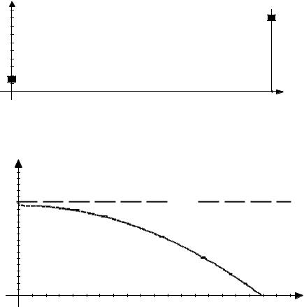
Fig. A1 - x(e) in case of binary effort e 0;1
1.08		b(1-m)
0.96							BC
0.84
0.72
0.6
0.48
0.36									IC
0.24
0.12											a
0		0.1	0.2	0.3	0.4	0.5	0.6	0.7	0.8	0.9	1

Fig. A2 – the actual bonus as a function of a

28

5		b
4.5
4
3.5
3								BC
2.5
2
1.5
1										IC
0.5											a
0		0.1	0.2	0.3	0.4	0.5	0.6	0.7	0.8	0.9	1
	Fig. A3 – BC with ρ=0.5, x(1)=0.9, x(0)=0.15

5	b
4.5
4
3.5						BC
3
2.5									IC
2
1.5
1
0.5
										a
0	0.1	0.2	0.3	0.4	0.5	0.6	0.7	0.8	0.9	1
	Fig. A4 – IC with (1) 0.74 ; other parameters are the same as in Fig.2

29