Lektsii (1) / Lecture 2

ICEF, 2012/2013 STATISTICS 1 year LECTURES

LECTURE 2

September, 11, 2012

3. Histogram (may be used for all types of data)

Example 1 (continued, discrete data). The die were tossed 20 times and the results are as follows

1	2	3	4	5	6
4 times	6 times	2 times	3 times	2 times	3 times

The picture is imported from Excel.

7
6
5
4
3
2
1
0
1	2	3	4	5	6

Fig. 4

The height of a bar is equal (proportional) to the corresponding number.

Example 2 (continued, continuous data)

1) The range of salaries is divided on the intervals with the length 5

	30
Частота	25
	20
	15
	10
	5
	0
	10 15	15 20	20 25	25 30	30 35	Еще

Fig. 5

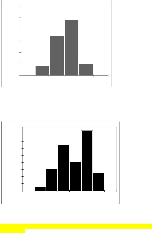
2) The range of salaries is divided on the intervals with the length 3

Частота	18
	16
	14
	12
	10
	8
	6
	4
	2
	0
	12-15	15-18	19-21	22-24	25-27	28-30	31-33	Еще

Fig. 6

The height of the bar is equal to the number of observation in the corresponding interval.

Important. For continuous data several histograms may be designed due to different selections of the intervals.

DESCRIPTIVE (SUMMARIZUNG) STATISTICS

(numerical data)

Let x1, x2 ,..., xn be some numerical data (distribution) not necessarily ordered.

Let Max = max{x1,..., xn }, Min = min{x1,..., xn } be the maximal and the minimal values of the

data set, respectively.

Definition 1. The number Range = Max −Min is called the range of the distribution

x1, x2 ,..., xn .
Example 2 (continued).
17.17	22.13	24.68	27.56	29.43
18.14	22.26	25.16	27.87	29.64
19.44	22.34	25.47	27.99	29.64
19.50	22.61	25.68	28.41	29.66
20.20	23.11	26.12	28.51	29.78
20.29	23.23	26.33	28.72	30.09
20.86	23.43	26.45	28.75	30.18
21.24	23.44	26.60	28.99	30.61
21.44	23.85	27.17	29.08	31.48
21.56	23.86	27.36	29.17	32.26
We have

Max =32.26, Min =17.17, Range =15.09 .

Definition 2. The number that separates 50% low observations and 50% upper observations is called the median of the distribution x1, x2 ,..., xn and is denoted med.

Median is a characteristic of a center of the distribution.

The median can be found by the following procedure.

•Sort the observations x1, x2 ,..., xn in ascending order and obtain a set x(1) ≤ x(2) ≤... ≤ x(n) . Important. You should understand that x(1) , x(2) ,..., x(n) are the same numbers as

x1, x2 ,..., xn but taking in different order. Particularly, x(1) = Min, x(n) = Max .

•If the number of observations n is odd, i.e. n = 2k +1 then med = x(k +1) .

•If the number of observations n is even, i.e. n = 2k then med = 12 (x(k ) + x(k +1) ) .

In the Example 2 we have n =50, x	= 26.12, x = 26.33, med = 26.12 +26.33		= 26.225
(25)	(26)	2

Exercise. How can a median be obtained (at lest, approximately) by using

(a)stem and leaf plot;

(b)*histogram?

Definition 3. The number that separates 25% low observations and 75% upper observations is called the low quartile (first quartile) of the distribution x1, x2 ,..., xn and is denoted LQ (Q1).

The number that separates 75% low observations and 25% upper observations is called the upper quartile (third quartile) of the distribution x1, x2 ,..., xn and is denoted UQ (Q3).

Definition 4. The number IQR =UQ −LQ is called interquartile range of the distribution x1, x2 ,..., xn .

IQR represents the spread or dispersion of 50% middle observations.

Exercise. Using Excel find LQ, UQ, IQR for the distribution of the previous example. В

русскоязычной версии Excel для этого надо использовать команду КВАРТИЛЬ. Целесообразно также посмотреть более общую команду ПЕРСЕНТИЛЬ.

In order to generalize the notions of median and quartile we introduce p−percentile.

Let number 0 < p <1 is given. Informally, p−percentile is the point that splits the distribution in such a way, that to the left of this point there is the share p of the total number of observations (n) while to the right − the share 1− p , respectively. Thus,

•median is 1/2−percentile,

•LQ is 1/4−percentile,

•UQ is 3/4−percentile.

Since the number np may be not integer we need some rule for calculating uniquely the

p−percentile.

Algorithm. In order to find the p−percentile one has to do the following

•To sort the distribution x1, x2 ,..., xn in ascending order and to obtain a set

x(1) ≤ x(2) ≤... ≤ x(n) .

•To get the presentation (n +1) p = k +a , where k an integer number and 0 ≤ a <1. Check that this can be uniquely done.

•To calculate the number x( p) = x(k ) +a (x(k +1) − x(k ) ) ; that is the p−percentile.

Example. Let n =66, p =0.2 . We have (n +1) p =67 0.2 =13.4 =13 +0.4 . Then

0.2 − percentile = x(13) +0.4 (x(14) − x(13) ) = 0.6 x(13) +0.4 x(14) .

Exercise. Check that x(k ) ≤ p − percentile ≤ x(k +1) .

		x + x +...+ x									1 n
Definition 5. The number x =		1				2			n	=	∑xi is called the sample mean of the
						n
											n i=1
distribution x1, x2 ,..., xn .
Sample mean is another characteristic of the center of the distribution x1, x2 ,..., xn .
Definition 6. The number s2 =		1				∑n		(xi −x )2			is called the sample variance of the distribution
			n −1 i=1
x1, x2 ,..., xn . The number s, i.e.		1					∑n		(xi −x )2 , is called the standard deviation of the
				n −1 i=1
distribution x1, x2 ,..., xn .

Variance and standard deviation are the characteristics of the spread or dispersion of a distribution.

The number di = xi − x is called deviation of the observation xi .

Exercise. Check that ∑n di =0 , i.e. the sum of all deviations is zero.

i=1

For the distribution of Example 2 we have x = 25.58, s2 =14.83, s =3.85 .

Remark. The reason of using denominator n −1, not n, in the definition of variance will be explained later.

Important. In practice the observations have some dimension, e.g., Rub, kg, cm, etc. Then median, quartiles, sample mean and standard deviation have the same dimension, while sample variance has the dimension of square of the dimension of the observations.