Lektsii (1) / Lecture 13

	ICEF, 2012/2013
	STATISTICS
	1 year
	LECTURES
Lecture 13	04.12.12

COVARIANCE AND CORRELATION

Let X and Y be two random variables with some joint distribution.

Definition. The number Cov(X ,Y ) = E ((X −µX )(Y −µY )) is called the covariance of the random variables X and Y where µX = E(X ), µY = E(Y ) .

We will also use the notation Cov(X ,Y ) =σXY /.

Proposition 1. Cov(X ,Y ) = E(X Y ) −µX µY .

Proof. Cov(X ,Y ) = E ((X −µX )(Y −µY ))= E(XY −µX Y −µY X + µX µY ) =

= E(XY ) −µX E(Y ) −µY E(X ) +µX µY = E(XY ) −µX µY ,	QED
It follows from the definition that Cov(X , X ) =V (X ) .

By direct calculation we get the following property of the covariance.

Proposition 2. Let X and Y be two random variables and a, b, c, d be some constants. Then

Cov(aX +b,cY +d ) = acCov(X ,Y ) .

Proposition 3. Let X and Y be two random variables. Then

V (X +Y ) =V (X ) +V (Y ) +2Cov(X ,Y ) .

Proof. We have

V (X +Y ) = E ((X −µX ) +(Y −µY ))2 = E ((X −µX )2 )+ E ((Y −µY )2 )+

+2E ((X −µX )(Y −µY ))=V (X ) +V (Y ) +2Cov(X ,Y ) , QED

Proposition 4. Let X and Y be two independent random variables. Then

E(X Y ) = E(X ) E(Y ) = µX µY .

Proof. We have (we use the standard notations from the previous lectures)

m n	m n	m		n
E(X Y ) = ∑∑xi y j pij = ∑∑xi y j pii		pi j = ∑xi pii		∑ y j pi j		=
i=1 j=1	i=1 j=1	i=1		j=1

m	m
= ∑xi pii µY	= µY ∑xi pii = µY µX ,	QED
i=1	i=1

Using Propositions 1, 4 we get

Proposition 5. If random variables X and Y are independent then Cov(X ,Y ) = 0 .

The inverse statement is not true, i.e. Cov(X ,Y ) = 0 does not imply independence of X and Y.

Proposition 6. If random variables X and Y are independent then V (X +Y ) =V (X ) +V (Y ) .

Since Cov(X ,Y ) has the dimension that is equal to the production of dimensions X and Y it

could not be used as a measure of “dependency” of X and Y. The modification of the covariance is the coefficient of correlation or simply correlation:

Definition. The number

	Corr(X ,Y ) =	Cov(X ,Y )	=		σXY
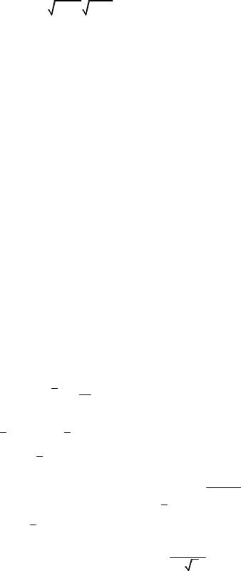
		V (X ) V (Y )		σX σY

is called the coefficient of correlation or simply correlation.

We will also use the notations Corr(X ,Y ) = ρXY = ρ(X ,Y ) .

Obviously correlation has no any dimension.

PROPERTIES OF CORRELATION

1.−1 ≤ ρ(X ,Y ) ≤1 for any random variables X and Y.

2.If random variables X and Y are independent then ρ(X ,Y ) = 0 .

3. If ρ(X ,Y ) =1 then there are constants a > 0 and b such that Y = aX +b ; if ρ(X ,Y ) = −1 then there are constants a < 0 and b such that Y = aX +b .

Random variables X and Y for which ρ(X ,Y ) = 0 are called uncorrelated. So, independent

random variables are independent but not vise versa.

The correlation is considered as a measure of linear relationships between X and Y.

LAW OF LARGE NUMBERS (LLN)

CENTRAL LIMIT THEOREM (CLT)

Let X1, X 2 ,... be an infinite sequence of independent and identically distributed random variables, E(Xi ) = µ, V (Xi ) =σ2 . Note that expectations and variances are the same for all random variables (why?). Let’s denote

Sn = ∑n Xi = X1 + X 2 +...+ X n − the sum of the first n terms of the sequence.

i=1

Obviously, E(Sn ) = n µ , and from Proposition 6 it follows that V (Sn ) = n σ2 . Finally, consider the random variables X(n) = Snn , n =1,2,... − the sequence of sample means of the first n terms of

the sequence. From the basic properties of expectation and variance it follows that

E (X(n) )= µ, V (X(n) )= σn2 .

Theorem (LLN). X(n) → µ as n →∞.

This statement is equivalent to the following statement: Sn −nnµ →0 as n →∞.

Informally this means that the randomness in X(n) disappears as n →∞. Intuitively it is quite clear because V (X(n) )→0 as n →∞.

Now consider the random variables Tn = Sσn −nnµ , n =1,2,... . It can be easily checked that

E(Tn ) = 0, V (Tn ) =1 .

Theorem (CLT). The distributions of random variables Tn tend to the distribution of the standard normal random variable Z as n →∞, i.e. Pr(a <Tn <b) → Pr(a < Z <b) for any a < b.

Particularly, the normal approximation can be applied to the binomial random variables. In fact, let Bn Bi(n,π) , then Bn is the total number of successes in n trials. Let’s introduce the random

0, if in i

th

trial false,

i =1,…, n.

variables εi =

1, if in ith trial success.

Then ε1,...,εn are independent and identically distributed random variables,

E(εi ) =π, V (εi ) =π(1−π) . Finally, Bn

= ∑n

εi , so we can use CLT for Bn :

i=1

The distribution of

Bn −nπ

tends to the distribution of a standard normal random

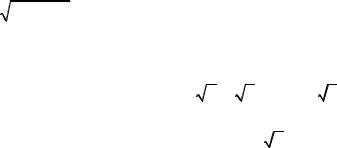
nπ(1−π)

variable Z.

Back to sample means. Since

(n) =

Sn

= µ +

Sn −nµ

σ

≈ µ +Z

σ

then for large n

X

n

n

n

σ n

(n) has approximately normal distribution N µ,

σ

whatever is the

the sample mean X

n

distribution of

X1, X 2 ,... .