Lektsii (1) / Lecture 4

ICEF, 2012/2013 STATISTICS 1 year LECTURES

LECTURE 4

25.09.2012

BACK TO HISTOGRAM: FREQUENCIES AND RELATIVE FREQUENCIES,

CUMULATIVE FREQUENCIES

Let x1, x2 ,..., xn be some distribution. Divide the whole domain of distribution by the intervals

∆1 =[a1,b1 ],..., ∆k	=[ak ,bk ] with equal widths and let
mj = #{xi	: xi ∆j ,i =1,..., n},					j =1,..., k ,
i.e. mj is the number of observations in the interval ∆j .
Definition. Numbers m1, m2 ,..., mk are called frequencies.
It must be clear that m1 +m2 +...+mk						= ∑k	mj = n .
						j =1
Definition. Numbers f j		=	mj	,	j =1,..., k are called relative frequencies.
			n
Clearly, f1 + f2 +...+ fk		= ∑k		f j	=1.
		j=1
Definition. Numbers cj		= f1 +...+ f j ,				j =1,..., k are called cumulative frequencies.

It immediately follows from the definition that

•c1 = f1, ck =1,

•c1 ≤c2 ≤... ≤ ck −1 ≤ ck ,

• f j = cj −cj−1, j = 2,..., k (check it!).

Remark. Since 0 ≤cj ≤1 cumulative frequencies are expressed sometimes in percents.

Using Excel we can construct the advanced histogram including cumulative frequencies (в

русскоязычной версии cumulative frequencies = интегральный процент).

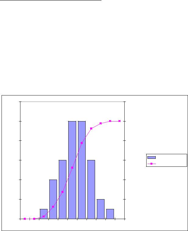
Example 4. The table below contains the incomes of 40 randomly selected people (thousands $, ascending order)

2.004	4.926	5.96	6.83
3.454	5.059	6.044	7.009
3.571	5.419	6.132	7.445
3.794	5.441	6.207	7.546
3.973	5.488	6.404	7.727
4.057	5.508	6.457	7.764
4.346	5.564	6.566	7.945
4.486	5.728	6.622	8.373

4.68	5.795	6.729	8.825
4.741	5.819	6.782	9.061

The table of frequencies and cumulative frequencies (imported from Excel)

Intervals	Frequency	Cumul. Frequency
0-1	0	0.00%
1-2	0	0.00%
2-3	1	2.50%
3-4	4	12.50%
4-5	6	27.50%
5-6	10	52.50%
6-7	10	77.50%
7-8	6	92.50%
8-9	2	97.50%
9-10	1	100.00%
> 10	0	100.00%

The histogram

Частот

12									120.00%
10									100.00%
8									80.00%
6									60.00%	Частота
										Интегральный%
4									40.00%
2									20.00%
0									0.00%
0-1	1-2	2-3	3-4	4-5	5-6	6-7	7-8	8-9	9-10 Еще

Fig. 7

Exercises

1.Using the histogram find (approximately) med, LQ, UQ of this distribution (Fig. 7).

2.Suppose that there are no any observations in some interval ∆j . What can you say about the

behavior of the cumulative frequencies curve?

COMPAROSON OF DISTRIBUTIONS

•back-to-back stem and leaf plots

•parallel box-plots

•up-and-down histograms

•parallel histograms

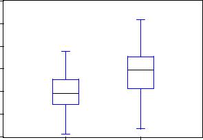
Below is the example of parallel box-plots:

18

16

14

12

10

8

6

X Y

From this picture we may conclude the following:

•the distribution Y is more “spread” than the distribution X: RangeX ≈7.7, RangeY ≈10.2 and IQRX < IQRY ;

•the distribution Y as whole may be considered as shifted up with respect to the distribution X.

Similarly the distributions could be compared by using histograms and stem-and-leaf plots.

Definition 10. For discrete data the most frequent value of the distribution x1, x2 ,..., xn is called the mode of the distribution. For continuous data the mode of the distribution x1, x2 ,..., xn is the point of maxima of the histogram.

In Example 1 (Fig. 4) the mode is 2. In Fig. 7 the mode is approximately 6 (see Lecture 3).

GROUPED DATA

Let x1, x2 ,..., xn be some distribution. Suppose that the data are grouped in the following way: there are m1 observations having the same value a1 ,

there are m2 observations having the same value a2 ,

…

there are mk observations having the same value ak .

Remind that according to Definition 7 the numbers mj , j =1,..., k are the frequencies. Then

x =	1 ∑n				xi = 1 (m1a1 +m2a2 +...+mk ak )= ∑k					f j a j	,
	n i=1					n			j=1
where f j =	mj			,	j =1,..., k are relative frequencies.
		n
Similarly (check it!)							n
s2 =	1				∑k	mj (a j − x )2 =		∑k	f j (a j − x )2 .
		n −1 j=1					n −1 j=1
If the number of observation is large or the only values a j											and relative frequencies f j are given,
then the variance should be calculated by the formula
s2 = ∑k				f j (a j − x )2 .
		j=1

CLUSTERS. Clusters are the natural subgroups into which the values of a distribution fall. GAPS. Gaps are the holes where no values fall.

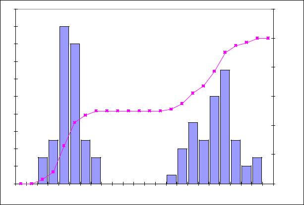
Example. Below is the histogram of teachers’ salaries in Moscow and in some small town (thousands Rub)

20																							120.00%
18
16																							100.00%
14																							80.00%
12
10																							60.00%
8
6																							40.00%
4																							20.00%
2
0																							0.00%
6	6.5	7	7.5	8	8.5	9	9.5	10	10.5	11	11.5	12	12.5	13	13.5	14	14.5	15	15.5	16	16.5	17	Еще

Obviously there are two clusters, around 8 and around 15, and there is gap between 10 and 12.5

THE TRANSFORMATION OF THE DESCRIPTIVE STATISTICS UNDER THE

TRANSFORMATIONS OF MEASURE UNITS

Example. Let x1,..., x20 be the height of 20 randomly selected people measured in cm. It is

known that

x =171, sx =15, medx =168 .

Suppose that the same observations are measured in feet. Denote this distribution y1,..., y20 . It is

known that

1 foot = 30.48 cm.

So, yi = 30.481 xi , i =1,...,20 , and

		1	20	1	20	x		1		1	20	1
	y =		∑yi =		∑	i	=				∑xi =		x =5.61.
		20		20		30.48		30.48		20		30.48
			i=1		i=1						i=1

Similarly

sy = 30.481 sx = 0.49, medy = 30.481 medx =5.51.

Exercise. Let the same observations are measured in two units and two distributions x1,..., xn and y1,..., yn , respectively, are obtained. The transformation from the first unit to the second is

described by

y = ax +b

where a and b are constants (in Example a = 301.48 , b = 0 ). Show that

(a)y = ax +b, sy =| a | sx , medy = a medx +b ,

(b)Find and prove similar formula for LQ,UQ, Range, IQR .

Self control

1. What is

•distribution

•numerical data

•discrete and continuous data (variables)

•ordered data

•qualitative (categorical) data

2. What is

•dot plot

•stem-and-leaf plot

•back-to-back stem-and-leaf plot

•histogram

•box plot

3. What is

•range

•low and upper quartiles

•median

•interquartile range

•sample mean

•sample variance

•standard deviation