DC14Sample

Copyright ©2007 by the Society for Industrial and Applied Mathematics.

This electronic version is for personal use and may not be duplicated or distributed.

6.2. Ziegler–Nichols Tuning Formula

193

Step Response

1.8

1.6← derivative in feedback

		1.4		← normal PID		proofs
		1.2
	Amplitude
		1
		0.8
		0.6
		0.4
		0.2
		0	0	5	10	15
				Time (sec)
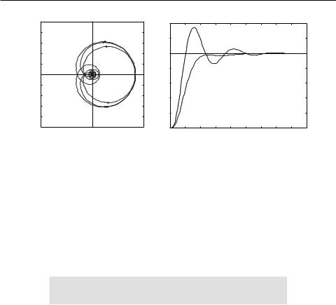
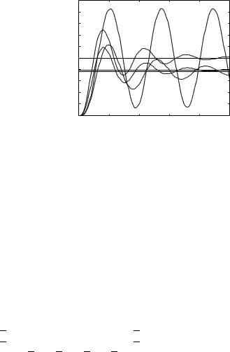
		Figure 6.10. PID controllers comparison.
The controllers designed are GPID(s) = 7.5600					(1 + 1/1.4050s + 0.3372s), with Kp		=
uncorrected
4.5360, Ti =	0.8430, Td		=	0.5620, and the step response comparison is shown in
Fig. 6.10(a).

It can be seen that although the PID controller with derivative in the feedback path might be easier and faster to be implemented compared to the normal PID controller, its performance may not be very satisfactory. Sometimes, such a PID controller should be designed using a dedicated algorithm to ensure a good control performance.

6.2.3 Methods for First-Order Plus Dead Time Model Fitting

It can be seen that the model (6.5) is useful for designing a PID controller because of the availability of a simple formula. The method in Sec. 6.2.1 for finding L and T of a given plant is simple to use with the graph of a plant step response. Although in modern computation it is not necessary to reduce a model to this form to find suitable PID controller parameters, which may be found by using the original model with one of many possible approaches, nevertheless it can be useful. Given the plant transfer function, we can use one of the model reduction methods described in Chapter 3. For example, the suboptimal reduction method [47] is very effective at the expense of an affordable heavy computational load. The optimal reduced-order model can be obtained with the function opt_app(), covered in Sec. 3.6. In this section, two other effective and frequently used algorithms will be introduced.

Frequency response method
Consider the frequency response of a first-order model
+				=		+
	k					k
G(jω) =	Ts	1	e−Ls s		jω =	T jω	1	e−jωL.	(6.9)

From "Linear Feedback Control" by Dingyu Xue, YangQuan Chen, and Derek P. Atherton.

This book is available for purchase at www.siam.org/catalog.

Copyright ©2007 by the Society for Industrial and Applied Mathematics.

This electronic version is for personal use and may not be duplicated or distributed.

194

Chapter 6. PID Controller Design

The ultimate gain Kc at the crossover frequency ωc is actually the first intersection of

a Nyquist plot with the negative part of the real axis, i.e.,

k(cos ωcL − ωcT sin ωcL)

1 ,

1 + ωc2T 2

= −

Kc

(6.10)

sin ω

c

L

ω

c

T cos ω L

0,

+

c

=

where k is the steady-state value or DC (direct current) gain of the system which can be

directly evaluated from the given transfer function. Define two variables x1 = L and x2 = T

satisfying

f1(x1, x2)

kKc(cos ωcx1 − ωcx2 sin ωcx1) + 1 + ωc2x22 = 0,

(6.11)

f2

(x1, x2)

= sin ωcx1

+

ωcx2 cos ωcx1

=

0.

=

The Jacobian matrix is that

∂f1/∂x1

∂f1/∂x2

J = ∂f2/∂x1

∂f2/∂x2

(6.12)

=

kK

ω

sin ω x

1−

kK

ω2x

cos ω

x

2ω2x

2 −

proofs

−

c

c

c

2 c

c

2

c

1

c

c

c

c

1 .

ωc cos ωcx1 −ωc x2 sin ωcx1

ωc cos ωcx1

So, (x1, x2) can be solved using any quasi-Newton algorithm. The MATLAB function

[K,L,T ]=

getfod(G)

is written for solving x1 and x2 in order to find the parameters

K, L, T of the

system.

function [K,L,T]=getfod(G,method)

2

K=dcgain(G);

3

if nargin==1

4

[Kc,Pm,wc,wcp]=margin(G); ikey=0; L=1.6*pi/(3*wc); T=0.5*Kc*K*L;

5

if finite(Kc), x0=[L;T];

6

while ikey==0, u=wc*x0(1); v=wc*x0(2);

7

FF=[K*Kc*(cos(u)-v*sin(u))+1+vˆ2; sin(u)+v*cos(u)];

8

J=[-K*Kc*wc*sin(u)-K*Kc*wc*v*cos(u), -K*Kc*wc*sin(u)+2*wc*v;

9

wc*cos(u)-wc*v*sin(u), wc*cos(u)];

x1=x0-inv(J)*FF;

if norm(x1-x0)<1e-8, ikey=1; else, x0=x1;

end, end

L=x0(1); T=x0(2);

end

elseif nargin==2 & method==1

[n1,d1]=tfderv(G.num{1},G.den{1}); [n2,d2]=tfderv(n1,d1);

K1=dcgain(n1,d1); K2=dcgain(n2,d2);

Tar=-K1/K; T=sqrt(K2/K-Tarˆ2); L=Tar-T;

end

function [e,f]=tfderv(b,a)

f=conv(a,a); na=length(a); nb=length(b);

e1=conv((nb-1:-1:1).*b(1:end-1),a);

e2=conv((na-1:-1:1).* a(1:end-1),b); maxL=max(length(e1),length(e2));

e=[zeros(1,maxL-length(e1)) e1]-[zeros(1,maxL-length(e2)) e2];

uncorrected

From "Linear Feedback Control" by Dingyu Xue, YangQuan Chen, and Derek P. Atherton.

This book is available for purchase at www.siam.org/catalog.

6.2. Ziegler–Nichols Tuning Formula

Copyright ©2007 by the Society for Industrial and Applied Mathematics.

This electronic version is for personal use and may not be duplicated or distributed.

195

Transfer function method

Consider the first-order model with delay given by

Gn(s) =

ke−Ls

.

Ts + 1

Taking the firstand second-order derivatives of Gn(s) with respect to s, one can immediate

find that

Gn(s)

T

Gn(s)

Gn(s)

2

T 2

= −L −

,

−

=

.

Gn(s)

1 + Ts

Gn(s)

Gn(s)

(1 + Ts)2

Evaluating the values at s = 0 yields

Tar = −

Gn(0)

2

=

Gn(0)

2

= L + T,

T

− Tar,

(6.13)

Gn(0)

Gn(0)

uncorrected

proofs

where Tar is also referred to as the average residence time. From the former equation, one has L = Tar − T . Again, the DC gain k can be evaluated from Gn(0).

The solution for the FOPDT model is thus obtained by using the derivatives of its transfer function G(s) in the above formula.

The MATLAB function getfod() listed earlier can be used with the syntax [K,L,T ]= getfod(G,1) to find the parameters K, L, T of the system.

Example 6.7. Consider the fourth-order model used in Example 6.4. The parameters of its approximate FOPTD model can be obtained using the MATLAB statements

>> G=tf(10,[1,10,35,50,24]);

[k,L,T]=getfod(G); G1=tf(k,[T 1]); G1.ioDelay=L; [Gc1,Kp3,Ti3,Td3]=ziegler(3,[k,L,T,10]) [k,L,T]=getfod(G,1), G2=tf(k,[T 1]); G2.ioDelay=L; nyquist(G,’-’,G1,’--’,G2,’:’); figure [Gc2,Kp4,Ti4,Td4]=ziegler(3,[k,L,T,10])

G c1=feedback(G*Gc1,1); G c2=feedback(G*Gc2,1); step(G_c1,G_c2)

The Nyquist plot comparisons of the plant model and the two approximations are shown in Fig. 6.11(a).

With the frequency response method, the K, L, T parameters are obtained as 0.4167, 0.7882, 2.3049. The PID controller designed with the Ziegler–Nichols formulas is Gc1(s) = 8.4219 (1 + 1/1.5764s + 0.3941s). While the parameters using the transfer function method are 0.4167, 0.8902, 1.1932, the PID controller is Gc2(s) = 3.8602 (1 + 1/1.7804s + 0.4451s). The closed-loop step responses with the above two PID controllers are shown in Fig. 6.11(b).

From "Linear Feedback Control" by Dingyu Xue, YangQuan Chen, and Derek P. Atherton.

This book is available for purchase at www.siam.org/catalog.

Copyright ©2007 by the Society for Industrial and Applied Mathematics.

This electronic version is for personal use and may not be duplicated or distributed.

196						Chapter 6.			PID Controller Design
		Nyquist Diagram						Step Response
	0.5			1.4
	0.4					← frequency response fitting
	0.3			1.2
	0.2			1
Imaginary Axis	0.1		Amplitude	0.8
	0
	−0.1			0.6		← transfer function based fitting
	−0.2			0.4
	−0.3
	−0.4			0.2
	−0.5	0	0.5	0	1	2	3	4	5	6	7	8	9
	−0.5			0
		Real Axis						Time (sec)
		(a) Nyquist plots			(b) closed-loop step responses
		Figure 6.11. PID controller responses.

It can be seen that although the PID controller designed with the transfer function identification algorithm looks better, it does not reflect the usual overshoot characteristics of Ziegler–Nichols tuning, presumably due to the inaccurately identified parameters of an

FOPDT model.	proofs
uncorrecteda 0 a − b

With the use of the suboptimal model reduction technique presented in Sec. 3.6.3, the parameters can be extracted with the following statements and the controller can better be

designed:

Gr=opt app(G,0,1,1); [n,d]=tfdata(G,’v’);

K=dcgain(G); T =d(1)/d(2); L=Gr.ioDelay;

6.2.4 A Modified Ziegler–Nichols Formula

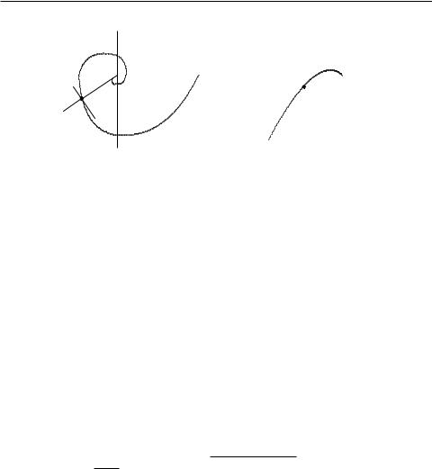
Consider the Nyquist frequency response shown in Fig. 6.12(a), where for a selected point A on the Nyquist plot, the control effects of the P, I, and D terms are shown in the appropriate directions. Thus, with properly chosen Kp, Ti, and Td , it is possible to move the given point A on the Nyquist curve of the uncontrolled plant to an arbitrary position on the Nyquist plot of the controlled system. The typical Nyquist plot under PID control is shown in Fig. 6.12(b), where A1 corresponds to the point A in Fig. 6.12(a).

	Denote pointAin the complex plane as G(jω0) = raej(π+φa). SupposeAis to be moved
to A1	which is represented by G1(jω0) = rb ej(π+φb). Assume that the PID controller at
frequency ω0 is Gc(s) = rcejφc . Then, obviously,
			rbej(π+φb) = rarcej(π+φa+φc).						(6.14)
Therefore, rc = rb/ra and φc			= φb − φa. So, based on the above analysis, PI and PID
controllers can be designed as follows:
•	PI control: The controller can be designed such that
	K		rb cos(φb − φa)	, T		1		,	(6.15)
		p =			i = ω tan(φ
			r				φ )

From "Linear Feedback Control" by Dingyu Xue, YangQuan Chen, and Derek P. Atherton.

This book is available for purchase at www.siam.org/catalog.

6.2. Ziegler–Nichols Tuning Formula

Copyright ©2007 by the Society for Industrial and Applied Mathematics.

This electronic version is for personal use and may not be duplicated or distributed.

197

Imaginary

Imaginary

real

real

I action

A

A1

P action D action

(a) original Nyquist plot

(b) new Nyquist plot

Figure 6.12. Sketches of FOPDT model.

which means that φa > φb for a positive Ti.

As a special case, the Ziegler–Nichols algorithm design is by

Kp = Kcrb cos φb,

Ti = −

Tc

,

(6.16)

2πtanφb

where Tc = 2π/ωc, ra = 1/Kc, and φa = 0.

proofs

• PID control: The controller can be designed such that

K

p =

rb cos(φb − φa)

,

ω

T

d −

1

=

tan(φ

b −

φ

).

(6.17)

ra

0

ω0Ti

a

uncorrected

Clearly, Ti and Td are not unique according to (6.17). To get a unique PID design, it

is a usual practice to set Td = αTi, where α is a constant. Given an α, Ti and Td can be obtained uniquely from

	1
Ti =	2αω0	tan(φb −φa)+ 4α+tan2(φb −φa) , Td = αTi.	(6.18)

By inspection, it is seen that the Ziegler–Nichols tuning formula is a special case when α = 1/4. The Ziegler–Nichols tuning formula can be rewritten as follows:

K

K r

cos φ

, T

i =

Tc

1+sin φb

, T

d =

Tc

1+sin φb

,

(6.19)

cos φb

4π

cos φb

p =

c

b

b

π

where ra = 1/Kc, φa = 0, and α = 1/4.

It can be seen that the PI or PID controllers can be designed by a suitable choice of rb and φb. The design problem is then one of selecting suitable values for these two parameters to give the appropriate performance. This is called a modified Ziegler–Nichols PI/PID tuning formula, which has been implemented in the MATLAB function ziegler(), too. The only difference is that vars = [Kc, Tc, rb, φb, N].

From "Linear Feedback Control" by Dingyu Xue, YangQuan Chen, and Derek P. Atherton.

This book is available for purchase at www.siam.org/catalog.

Copyright ©2007 by the Society for Industrial and Applied Mathematics.

This electronic version is for personal use and may not be duplicated or distributed.

198	Chapter 6. PID Controller Design

		Step Response									Step Response
	1.6								1.5
	1.4	← φb = 10◦									← Ziegler-Nichols PID
Amplitude	1.2							Amplitude
	1								1
	0.8	←	φb	=	70◦
	0.6
									0.5
											← rb = 1
	0.4
	0.2
	0	5		10		15	20		0	2	4	6	8	10
	0								0
			Time (sec)								Time (sec)
		(a) for different φb									(b) for different rb
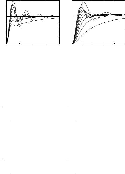
			Figure 6.13. Closed-loop step responses.
Example 6.8. Consider the plant model given by G(s) = 1/(s + 1)3. The PID controller
by the original Ziegler–Nichols tuning method can be obtained as follows:
>> G=tf(1,[1,3,3,1]); [Kc,pp,wg,wp]=margin(G); Tc=2*pi/wg;
[Gc1,Kp1,Ti1,Td1]=ziegler(3,[Kc,Tc,10])
and the controller G(s)											proofs
				= 4.8007 (1 + 1/1.8137s + 0.4353s) is obtained.									Now, let us
illustrate the flexibility of the modified Ziegler–Nichols PI/PID tuning formula. First, fix
rb = 0.5 and change φb. By the following MATLAB statements:

>>G c=feedback(G*Gc1,1); step(G c,20); rb=0.5; hold on for pb=[10:10:70]

[Gc2,Kp2,Ti2,Td2]=ziegler(3,[Kc,Tc,rb,pb,10]); G c2=feedback(G*Gc2,1); step(G c2,20);

end

the closed-loop step responses of the system for different values of φb are shown in Fig. 6.13(a). Clearly, when φb increases, the overshoot and oscillation become smaller. When φb is larger than 60◦, there is no overshoot, but the response becomes too sluggish. A good choice for the phase angle based on these responses is approximately 45◦.

Now, fix φb at φb = 45◦ and change rb. By the MATLAB statements

>>G c=feedback(G*Gc1,1); step(G c,10); pb=45; hold on; for rb=[0.1:0.1:1]

[Gc2,Kp2,Ti2,Td2]=ziegler(3,[Kc,Tc,rb,pb,10]); G c2=feedback(G*Gc2,1); step(G c2,10);

end

uncorrectedthe closed-loop step responses of the system for different rb are compared in Fig. 6.13(b). It can be seen that the smaller the rb, the smaller the overshoot and the slower the response.

Clearly, rb = 0.45, and φb = 45◦ can be considered as a good choice for this example with almost no overshoot and with a reasonably fast response.

It can be concluded that the modified tuning method is advantageous over the original Ziegler–Nichols PI/PID tuning technique.

From "Linear Feedback Control" by Dingyu Xue, YangQuan Chen, and Derek P. Atherton.

This book is available for purchase at www.siam.org/catalog.

Copyright ©2007 by the Society for Industrial and Applied Mathematics.

This electronic version is for personal use and may not be duplicated or distributed.

6.3. Other PID Controller Tuning Formulae

199

6.3 Other PID Controller Tuning Formulae

Many variants of the traditional Ziegler–Nichols PID tuning methods have been proposed. Several of these are given in the following section.

6.3.1 Chien–Hrones–Reswick PID Tuning Algorithm

The Chien–Hrones–Reswick (CHR) method [66] emphasizes the set-point regulation or disturbance rejection. In addition one qualitative specifications on the response speed and overshoot can be accommodated. Compared with the traditional Ziegler–Nichols tuning formula, the CHR method uses the time constant T of the plant explicitly.

The CHR PID controller tuning formulas are summarized in Table 6.2 for set-point regulation. The more heavily damped closed-loop response, which ensures, for the ideal plant model, the “quickest response without overshoot” is labeled “with 0% overshoot,” and the “quickest response with 20% overshoot” is labeled “with 20% overshoot.”

Similarly, Table 6.3 is used to design controllers for disturbance rejection purposes. A MATLAB function chrPID() is written which can be used to design different

controllers using the CHR algorithms:

function [Gc,Kp,Ti,Td,H]=chrpid(key,tt,vars)

proofs

2

K=vars(1); L=vars(2); T=vars(3); N=vars(4); a=K*L/T; Ti=[]; Td=[];

3

ovshoot=vars(5); if tt==1, TT=T; else TT=L; tt=2;

end

4

if ovshoot==0,

5

KK=[0.3,0.35,1.2,0.6,1,0.5; 0.3,0.6,4,0.95,2.4,0.42];

6

else,

7

KK=[0.7,0.6,1,0.95,1.4,0.47; 0.7,0.7,2.3,1.2,2,0.42];

8

end

9

switch key

case 1, Kp=KK(tt,1)/a;

case 2, Kp=KK(tt,2)/a; Ti=KK(tt,3)*TT;

case {3,4}, Kp=KK(tt,4)/a; Ti=KK(tt,5)*TT; Td=KK(tt,6)*L;

end

[Gc,H]=writepid(Kp,Ti,Td,N,key);

Table 6.2. CHR tuning formulae for set-point regulation.

Controller

with 0% overshoot

with 20% overshoot

type

Kp

Ti

Td

Kp

Ti

Td

P

0.3/a

0.7/a

PI

0.35/a

1.2T

0.6/a

T

PID

0.6/a

T

0.5L

0.95/a

1.4T

0.47L

Table 6.3. CHR tuning formulae for disturbance rejection.

Controller

with 0% overshoot

with 20% overshoot

type

Kp

Ti

Td

Kp

Ti

Td

P

0.3/a

0.7/a

PI

0.6/a

4L

0.7/a

2.3L

PID

0.95/a

2.4L

0.42L

1.2/a

2L

0.42L

uncorrected

From "Linear Feedback Control" by Dingyu Xue, YangQuan Chen, and Derek P. Atherton.

This book is available for purchase at www.siam.org/catalog.

Copyright ©2007 by the Society for Industrial and Applied Mathematics.

This electronic version is for personal use and may not be duplicated or distributed.

200			Chapter 6. PID Controller Design
	The syntax of the chrpid() function is
		[Gc,Kp,Ti,Td ]=chrPID(key,typ,vars)
			proofs
where the returned variables are defined similar to those in ziegler(). key = 1, 2, 3
is for P, PI, and PID controllers, respectively. The variable typ denotes the type of criteria
used with typ = 1 for set-point control and any other value for disturbance rejection.
vars = [k, L, T, N, Os] with Os = 0 denotes no overshoot, and any other value denotes
20% overshoot.

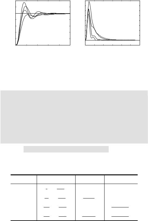
Example 6.9. Consider the plant model in Example 6.4. The Ziegler–Nichols PID controller and the four CHR controllers for different controller types and specifications are obtained using the following statements:

>> s=tf(’s’); G=10/((s+1)*(s+2)*(s+3)*(s+4)); [k,L,T]=getfod(G); N=10; [Gc1,Kp,Ti,Td]=ziegler(3,[k,L,T,N])

[Gc2,Kp,Ti,Td]=chrpid(3,1,[k,L,T,N,0])
uncorrected
[Gc3,Kp,Ti,Td]=chrpid(3,1,[k,L,T,N,20])
[Gc4,Kp,Ti,Td]=chrpid(3,2,[k,L,T,N,0]);
The four PID controllers designed are, respectively,
G1(s) = 8.4219 1+	1	+0.3941s , G2(s) = 4.2110 1	+	1	+0.3941s ,
	1.5764s			2.3049s
G3(s) = 6.6674 1+	1	+0.3704s , G4(s) = 6.6674 1	+	1	+0.3310s .
	3.2268s			1.8917s

For the different controllers designed in the above, the step response of the closed-loop systems can be obtained using the following MATLAB statements:

>> step(feedback(G*Gc1,1),feedback(G*Gc2,1),feedback(G*Gc3,1),...

feedback(G*Gc4,1),10)

as summarized in Fig. 6.14(a). It can be seen that the set-point regulation controller with 0% overshoot gives a satisfactory result. Similarly, with the following MATLAB statements:

>> step(feedback(G,Gc1),feedback(G,Gc2),feedback(G,Gc3),...

feedback(G,Gc4),30)

the closed-loop responses to a step disturbance signal can be obtained as shown in Fig. 6.14(b). Clearly, compared with the traditional Ziegler–Nichols controller, the effect of the disturbance signal can be significantly reduced by a CHR controller.

6.3.2 Cohen–Coon Tuning Algorithm

Another Ziegler–Nichols type tuning algorithm is the Cohen–Coon tuning formula [67]. Referring to the FOPDT model (6.5) approximately obtained from experiments, denote

From "Linear Feedback Control" by Dingyu Xue, YangQuan Chen, and Derek P. Atherton.

This book is available for purchase at www.siam.org/catalog.

Copyright ©2007 by the Society for Industrial and Applied Mathematics.

This electronic version is for personal use and may not be duplicated or distributed.

6.3. Other PID Controller Tuning Formulae

201

				Step Response												Step Response
		1.4											0.16
		1.2											0.14
													0.12
		1											0.1
	Amplitude											Amplitude
		0.8											0.08
		0.6											0.06
		0.4											0.04
													0.02
		0.2											0
		0	2	4	6					8	10		−0.02	5	10	15	20	25	30
		0											0
				Time (sec)												Time (sec)
			(a) set-point step response											(b) disturbance step response
			Figure 6.14. Closed-loop step responses of CHR controllers.
	a = kL/T and τ = L/(L + T). The different controllers can be designed by the direct use
	of Table 6.4.
		A MATLAB function cohenpid() is written which can be used to design a PID
	controller using the Cohen–Coon tuning formulas:														proofs
	function [Gc,Kp,Ti,Td,H]=cohenpid(key,vars)
2	K=vars(1); L=vars(2); T=vars(3); N=vars(4);
3	a=K*L/T; tau=L/(L+T); Ti=[]; Td=[];
4	switch key
5 case 1,Kp=(1+0.35*tau/(1-tau))/a;
6	case 2,
7	Kp=0.9*(1+0.92*tau/(1-tau))/a; Ti=(3.3-3*tau)*L/(1+1.2*tau);
8	case {3,4}, Kp=1.35*(1+0.18*tau/(1-tau))/a;
9	Ti=(2.5-2*tau)*L/(1-0.39*tau); Td=0.37*(1-tau)*L/(1-0.81*tau);
	case 5
	Kp=1.24*(1+0.13*tau/(1-tau))/a; Td=(0.27-0.36*tau)*L/(1-0.87*tau);
	end
	[Gc,H]=writepid(Kp,Ti,Td,N,key);
	The syntax is		[Gc,Kp,Ti,Td ,H]=cohenpid(key,vars) , where the vars argu-
	ments should be written as vars = [k, L, T, N].
			Table 6.4. Controller parameters of Cohen–Coon method.
		Controller						Kp						Ti			Td
				1					0.35τ
			P	a	1 + 1 − τ								3.3 − 3τ L
			PI	0.9		1		+		0.92τ
				a						1 − τ			1 + 1.2τ
		PD		1.24			1		+	0.13τ						0.27 − 0.36τ L
				a						1 − τ						1 − 0.87τ
		PID		1.35			1		+	0.18τ			2.5 − 2τ L			0.37 − 0.37τ L
				a						1 − τ			1 − 0.39τ			1 − 0.81τ
uncorrected

From "Linear Feedback Control" by Dingyu Xue, YangQuan Chen, and Derek P. Atherton. This book is available for purchase at www.siam.org/catalog.

Copyright ©2007 by the Society for Industrial and Applied Mathematics.

This electronic version is for personal use and may not be duplicated or distributed.

202	Chapter 6. PID Controller Design

Step Response

2

1.8← PI

	1.6
Amplitude	1.4	← PID
	1.2	← P
	1
	0.8		← PD
	0.6
	0.4
	0.2
	0	2	4	6	8	10
	0
				Time (sec)
Figure 6.15. Step responses under controllers of the Cohen–Coon method.

>> G=tf(10,[1,10,35,50,24]); [k,L,T]=getfod(G);

Example 6.10. Consider the plant model given in Example 6.4proofswith its P, PI, PD, and PID controllers designed using the following MATLAB statements:

[Gc1,Kp1]=cohenpid(1,[k,L,T,10])

[Gc2,Kp2,Ti2]=cohenpid(2,[k,L,T,10])

[Gc3,Kp3,Ti3,Td3]=cohenpid(5,[k,L,T,10])

[Gc4,Kp4,Ti4,Td4]=cohenpid(3,[k,L,T,10])

and the controllers are obtained as

G1(s) = 7.8583, G2(s) = 8.3036 (1 + 1/1.5305s) ,

G3(s) = 9.0895(1 + 0.1805s), G4(s) = 10.0579 (1 + 1/1.7419s + 0.2738s) .

With the following MATLAB statements:

>> G c1=feedback(G*Gc1,1); G c2=feedback(G*Gc2,1); G c3=feedback(G*Gc3,1); G c4=feedback(G*Gc4,1); step(G c1,G c2,G c3,G c4,10)

the closed-loop step responses of the systems with the different controllers are shown in Fig. 6.15.

6.3.3 Refined Ziegler–Nichols Tuning

Since the PID controller designed by the conventional Ziegler–Nichols tuning formulas often exhibits rather strong oscillation in the set-point response and a large overshoot, a refinement to such a PID controller tuning algorithm can be obtained with the use of setpoint weighting [68]:

	1			dy
u(t) = Kp	(βuc − y) +		edt − Td		, (6.20)
		Ti		dt
uncorrected

From "Linear Feedback Control" by Dingyu Xue, YangQuan Chen, and Derek P. Atherton.

This book is available for purchase at www.siam.org/catalog.