LECTURE #5

Current size of Genbank (June 2011): 129,178,292,958 bp (1.3 x 1011, or 129 tera-base pairs) in 140,482,268 entries. This doesn’t include unprocessed genomic sequences, which would double the size.

This would be hard to deal with if it were all written on pieces of paper stored in file cabinets.

In 1982, Genbank contained 690,338 bp in 606 entries, which fit on two 5 ¼ inch floppy disks (360 kB capacity), which Genbank mailed to you.

At its simplest, a database is a way to store information and retrieve it efficiently.

However, nearly all databases add value to the information by processing it in different ways.

Biological databases: Why?

Make biological data available to scientists

Consolidation of data (gather data from different sources)

Provide access to large dataset that cannot be published explicitly (genome, …)

Make biological data available in computer-readable format

Make data accessible for automated analysis

Bioinformatics: “a collective term for data compilation, organisation, analysis and dissemination”

Database Background

The general concepts of storing and retrieving data go back to very beginnings of writing.

How to record data in a uniform fashion, and how to file it where you can find it again later. Concepts like:

forms,

alphabetical order,

serial numbers,

filing cabinets with separate drawers and folders within drawers

Use of machines to accurately tabulate information (typewriter, adding machine, etc.)

Computers allowed even larger amounts of information to be stored

Computers are like being blind: they

Sumerian land purchase records from about 2400 BCE

Some Common Databases

European Molecular Biology Laboratory http://www.ebi.ac.uk/Information/

DNA Database of Japan http://www.ddbj.nig.ac.jp/

Discover http://discover.nci.nih.gov/

Oncomine 3.0 http://www.oncomine.org/main/index.jsp

Gene Expression Omnibus http://www.ncbi.nlm.nih.gov/geo/

CGAP/SAGE http://cgap.nci.nih.gov/

Codd’s Normal Forms

In 1970, IBM researcher E. F. Codd published the seminal paper “A relational model of data for large shared data banks”, which specified the basic design principles still used today for designing databases.

“relational” databases, that is. There are other ways of doing databases, not as widely used.

Codd’s fundamental insight was to put data into multiple tables connected together by unique keys. This is opposed to the typical spreadsheet idea of having all the data together in one big table.

Making a database adhere to Codd’s principals is called “normalization”, and the principles themselves are called “normal forms”.

At present there are 6-8 normal forms: defining them is part of database theoretical research. “relational algebra”

Databases that conform to the normal forms are:

Easy and fast to search, and give the correct unique results

Easy to update: each piece of data is stored in a single locationEasy to extend to new types of data

Basic Structure

Databases are composed of tables of data.

Tables hold logically related sets of data. A table is essentially the same thing as a spreadsheet: a set of rows and columns.

Each table has several records:

a record stores all the information for a given individual

Records are the rows of a data table

Each record has several fields:

A field is an individual piece of data, a single attribute of the record.

Fields are the columns of a data table

Each record (row) has a unique identifier, the primary key.

the primary key serves to identify the data stored in this record across all the tables in the database.

Databases are manipulated with a language called SQL (Structured Query Language). It’s a “baby English” type of language: uses real words, but rigid in terms of the order and placement.

Various database software: Oracle, MS Access, MySQL, etc.

Indexing

A database index is a data structure that improves the speed of data retrieval, but at a cost of slower changes to the data and increased storage space.

Any column (field) of any table can be indexed. The index is just a list of which records (rows) have given values for that field.

You make an index that matches a frequent query. For instance, “which company belong to which client?”

Indexed on “species” column

feline : 1, 2, 3, 6 canine: 4, 7, 8, 10, 11 avian: 5

reptile: 9

Indexed on “client_id” column

1:1, 2, 3

2:4

3:5

4:6

5:7, 8

6:9, 10

7:11

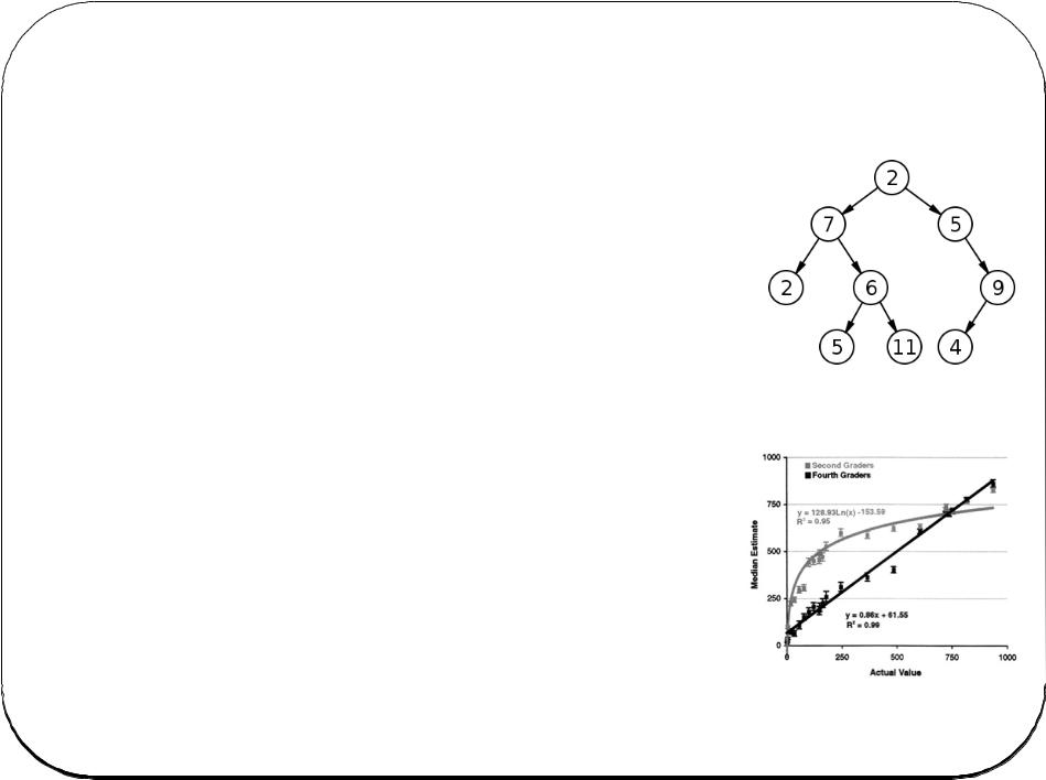
Search Trees

From the computer’s point of view, the simplest way to find a given record in a file is to start at the beginning of the file and read every record until it finds the right one.

This is obviously not very efficient for big files.

It is much faster to keep the file sorted, and then search it in a binary fashion: as with finding a word in a dictionary.

The basic concept is the binary tree. You find a given record by dividing the problem into halves repeatedly.

To find “tree” in the dictionary, you open it halfway, then determine your word is in the second half, then open that part at the halfway point, etc.

This is efficient: on average you look at logN records with a binary tree, and N/2 records with a linear search, where N is the number of records.

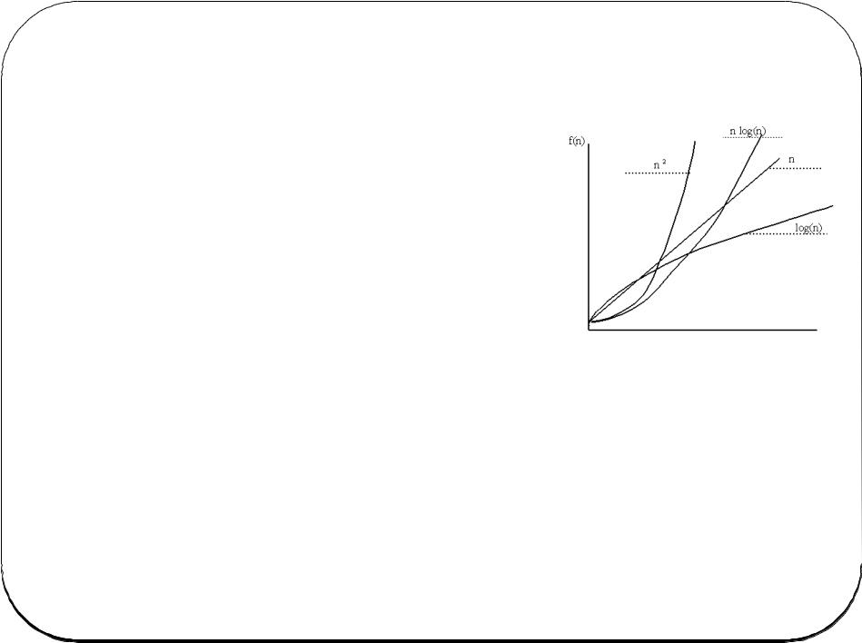
Computational Complexity

Different programs use different amounts of time, computer memory, number of calculations, etc., which greatly affect your ability to get results.

Time, space, and number of computations are all interrelated.

“Big O notation” is a way of quantifying this. The basic idea is how does the time, space, complexity scale with the number of objects being examined (n)?

O(1) = constant time. E.g. determine whether a number is even or odd.

O(log n) = logarithmic time. E.g. binary search

O(n) – linear time. E.g. finding something in an unsorted list

O(n log n). E.g. fast sorting algorithms

O(n2). Quadratic time. Simple sorting “bubble sort”

Travelling salesman

problem:

--how to plan a route between many cities minimizing the total distance travelled --trying all possibilities: the number increases exponentially

--going to the closest remaining city each time doesn’t work.

The different types of Databases in Bioinformatics

1) Data:

Type of data:

•nucleotide sequences

•protein sequences

•3D structures

•gene expression data

•metabolic pathways

•….

Data entry and quality control:

•data deposited directly

•curators add and update data

•treatment of erroneous data: removed, or marked

•error checking

•consistency, updates

•….

Primary, or derived data:

•Primary databases: direct experimental results

•Secondary databases: result of analysis on primary databases

•Consolidation of many databases

•…