Bologna / 02_TCAD_laboratory_A_simulation_primer_GBB_20140326H1020

Technology Computer Aided

Design (TCAD) Laboratory

Lecture 2,

A simulation primer

[Source: Synopsys]

Giovanni Betti Beneventi

E-mail: [e-mail] ; [e-mail]

Office: Engineering faculty, ARCES lab. (Ex. 3.2 room), viale del Risorgimento 2, Bologna Phone: [phone]

Advanced Research Center on Electronic Systems (ARCES) University of Bologna, Italy

G. Betti Beneventi

1

Outline

•Introduction

•Definition of equilibrium and out-of-equilibrium

•Static, Transient and AC simulations

•Simplify the simulation domain

•Numerical methods from a TCAD user perspective

•Meshing

•Numerical methods

•Synopsys Sentaurus TCAD Solvers

G. Betti Beneventi

2

Outline

 Introduction

•Definition of equilibrium and out-of-equilibrium

•Static, Transient and AC simulations

•Simplify the simulation domain

•Numerical methods from a TCAD user perspective

•Meshing

•Numerical methods

•Synopsys Sentaurus TCAD Solvers

G. Betti Beneventi

3

Introduction

•In this lecture we will talk about different topics, all of them to be discussed before starting the laboratory activity.

•Some content of this class is related to the review of basic concepts, like the choice of a simulation domain, the equilibrium and out-of-equilibrium definitions, the definitions of static, transient, and AC simulations.

•In addition, a TCAD user perspective background on the numerical methods and on the solvers used in Synopsys Sentaurus TCAD is provided.

G. Betti Beneventi

4

Outline

• Introduction

Definition of equilibrium and out-of- equilibrium

•Static, Transient and AC simulations

•Simplify the simulation domain

•Numerical methods from a TCAD user perspective

•Meshing

•Numerical methods

•Synopsys Sentaurus TCAD Solvers

G. Betti Beneventi

5

Equilibrium and out-of-equilibrium

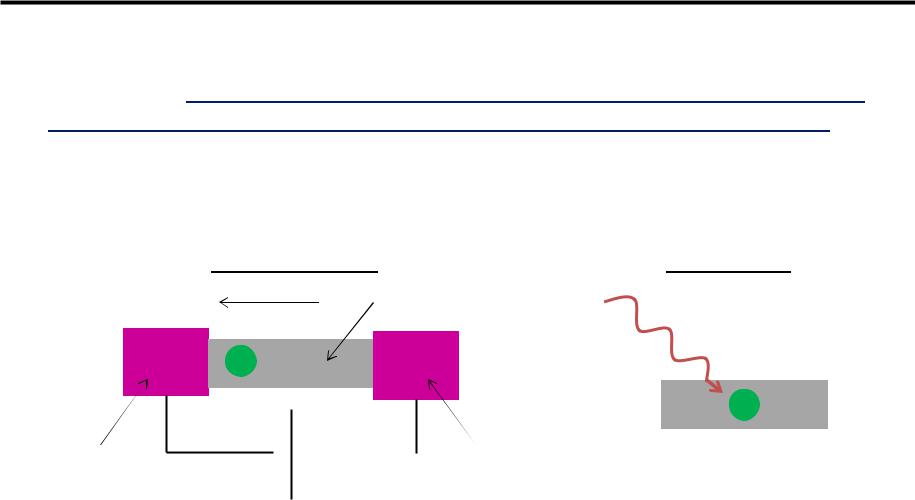
•In a system under equilibrium condition, each process and its inverse must selfbalance independently from any other process that may occur in the system. In other words, equilibrium is the special case where each fundamental process and its inverse self-balance, it is also known as detailed balance principle.

•If a net current flows, or if light is shined upon the semiconductor creating free carriers, we are out-of-equilibrium.

Applied Voltage

Shined light

I semiconductor

E= hν

e

e

electrode				electrode
			V

•A system under steady-state, transient, or ac signal is always out-of-equilibrium. The only exception is the presence of a capacitor, than can be biased but in which the net current flow is zero due to the presence of the oxide

G. Betti Beneventi

6

Outline

•Introduction

•Definition of equilibrium and out-of-equilibrium

 Static, Transient and AC simulations

•Simplify the simulation domain

•Numerical methods from a TCAD user perspective

•Meshing

•Numerical methods

•Synopsys Sentaurus TCAD Solvers

G. Betti Beneventi

7

Static, transient, and AC simulations (1)

•Static condition or steady-state (DC bias point). In steady-state conditions, for each property of the systems, its partial derivative with respect to time is zero, i.e. , nothing is changing with time.

•To perform steady-state simulations, the Sentaurus TCAD keyword is

Quasistationary. The Quasistationary command is used to ramp a

device from a solution to another through the modification of the boundary conditions (that can be Voltage, Current, or Temperature).

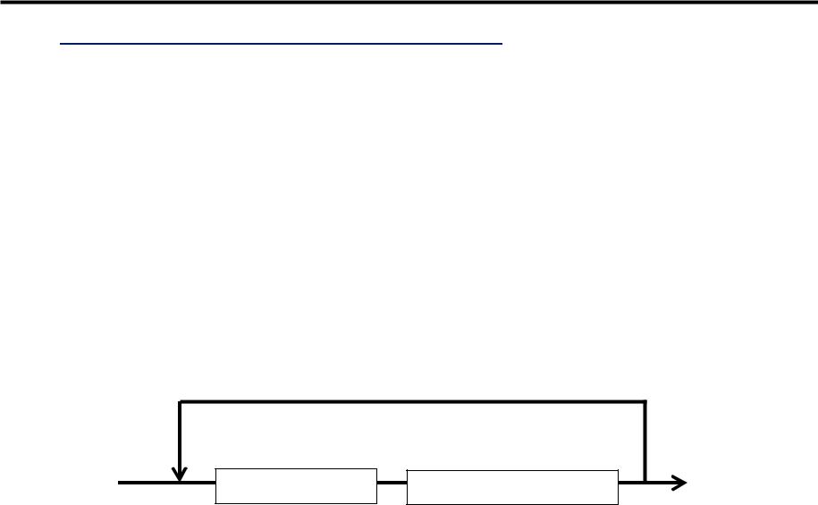
•For example, ramping a drain voltage of a device from 0 to 5V is performed by

Quasistationary( Goal {Voltage=5 Name=Drain } ){

Coupled { Poisson Electron Hole } }

Step Boundary

Re-solve the Device

G. Betti Beneventi

8

Static, transient, and AC simulations (2)

•Transient response. A transient response or natural response is the timevarying response of a system to a change from equilibrium.

•In Sentaurus, the keyword that must be used to perform transient simulation is Transient. The command must start with a device that has already been solved under stationary conditions. The simulation then proceeds by iterating between incrementing time and re-solving the device.

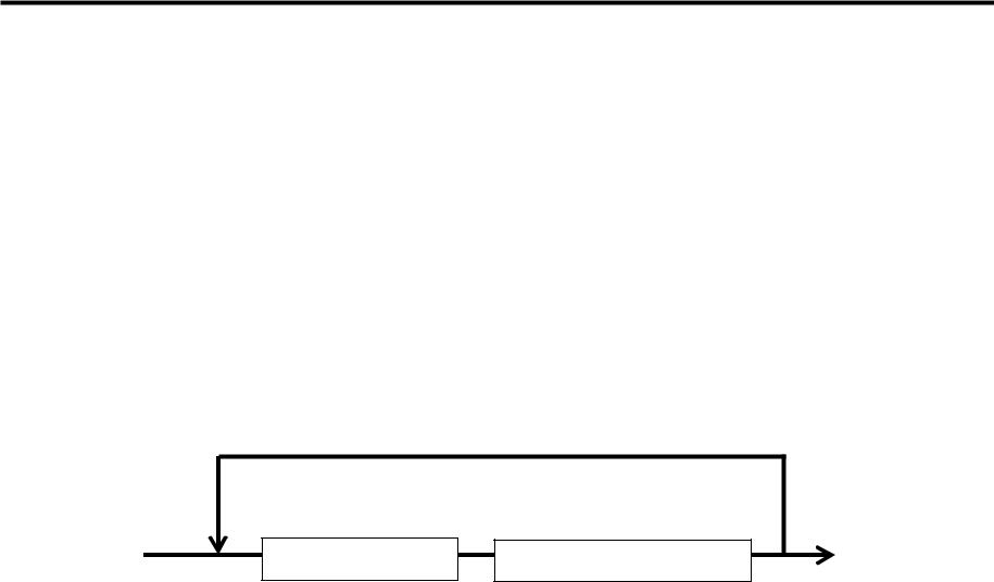
•An example of performing a transient simulation is:

Transient( InitialTime = 0.0 FinalTime=1.0e-5 ){

Coupled { Poisson Electron Hole }

}

Increment time

Re-solve the Device

G. Betti Beneventi

9

Static, transient, and AC simulations (3)

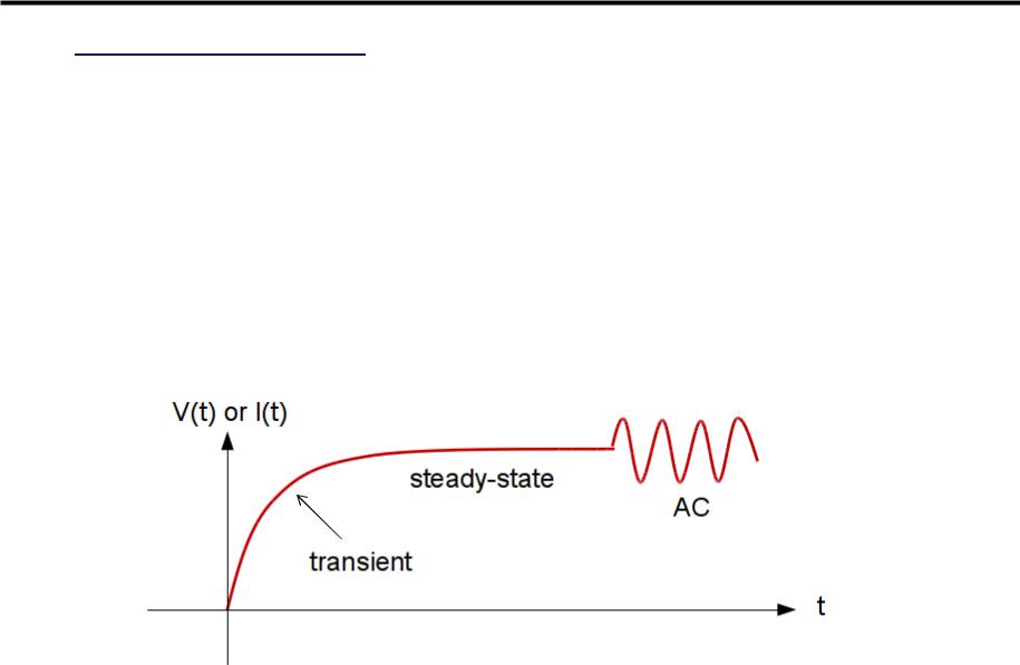
•Small signal AC analysis. Performing a small signal or AC analysis means simulate the behavior of system when a relatively small harmonic signal is superimposed to a steady-state condition or DC bias point.

•Small-signal modeling is a common analysis technique in electrical engineering which is used to approximate the behavior of nonlinear devices with linear equations. This linearization is formed about the DC bias point of the device (that is, the voltage/current levels present when no AC signal is applied), and can be accurate for small excursions about this point.

•The keyword for AC analysis in Sentaurus Sdevice is ACCoupled.

Graphical, qualitative, illustration of steady-state, transient, and AC signals.

G. Betti Beneventi 10