Fundamentals of the Physics of Solids / 10-The Structure of Noncrystalline Solids

10

The Structure of Noncrystalline Solids

We started our investigation into solid-state physics with the statement that in thermal equilibrium at low temperatures atoms in a solid are expected to be arranged in a regular periodic array, and so solids are characterized by a long-range positional order. However, it has been known for a long time that there exist certain materials that can be considered as solids from a mechanical point of view although the atomic arrangement in them is disordered as in liquids. They only exhibit short-range order, if any. It has also been shown recently that certain solids may have a state with some kind of long-range order even though atoms are not arranged periodically. In the present chapter we shall discuss the structural characteristics of such materials.

10.1 The Structure of Amorphous Materials

In solids prepared from melts by quenching, cooling may be so rapid that it leaves no time for nucleation and crystal growth, and so the equilibrium crystalline phase is not reached. Atoms freeze into a disordered, thermodynamically metastable state that is similar to the liquid phase or to a glassy (vitreous) state.

Similar structures are formed when atoms are evaporated on a surface, and randomly arriving atoms are stacked on top of each other in a disordered way. Solid, mechanically rigid materials in which atoms are arranged randomly are called amorphous.1 No long-range positional order exists inside them but they may exhibit short-range order.

10.1.1 Models of Topological Disorder

Two simple models for the structure of disordered materials are worth mentioning. In the first one atoms considered as rigid spheres are packed randomly

1Amorphous metallic materials produced by quenching alloys that are close to their eutectic points are also called metallic glasses.

304 10 The Structure of Noncrystalline Solids

but as tightly as possible. This dense random packing model is in fact the extension of the Bernal model of liquids to the amorphous, glassy state. This is illustrated in two dimensions in Fig. 2.2, where the plane is covered with randomly arranged but touching circles.

This can be used to model the structure of amorphous materials in which atoms have a repulsive core but otherwise tend to approach each other as much as possible. This is usually the case for metals – which explains why hexagonal close-packed and face-centered cubic structures occur so often in metals. In amorphous metals short-range order is due to this tendency for close packing. As we have seen, in close-packed fcc and hcp crystals each atomic sphere touches 12 neighbors, giving a packing fraction of almost 75%. In randomly packed structures – even when spheres touch as many others as possible – space filling is less e cient than in regular lattices. Empirical evidence shows that the packing fraction is at most 64%; on the average each sphere touches 8 to 9 others. A somewhat better space filling is obtained in numerical simulations when the randomly placed but touching atomic spheres are allowed small displacements toward local energy minima in their respective potential fields due to the other atoms (i.e., along the direction of the gradient of the full potential felt by the atom).

The other model, which leads to much less e cient space filling, is applicable to covalently bonded systems. In Chapters 4 and 7 we saw that covalent bonds are highly directional, and fix the relative orientation of nearestneighbor atoms. A prime example was the diamond structure in which each atom is surrounded by four neighbors in a unique tetrahedral arrangement. The crystal structure can be considered as the network of such bonds. Relative orientation of the tetrahedra plays a key role in forming the structure. The wurtzite and sphalerite structures of zinc sulfide (ZnS) di er precisely in the relative orientation of the tetrahedra. Similar tetrahedral geometry is observed in quartz (SiO2). Around each silicon atom oxygen atoms are placed in the directions of the four vertices of a tetrahedron. Joined at their vertices, these tetrahedra make up a three-dimensional network. Since neighboring tetrahedra may easily rotate with respect to one another, quartz often appears in an amorphous state.

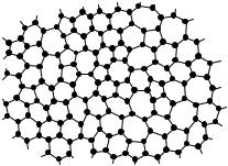
In Fig. 7.16 showing diamond and sphalerite structures tetrahedral bonds are seen to form hexagonal rings. When the tetrahedra are rotated, there is a finite probability for a ring to contain seven or five rather than six atoms. A two-dimensional illustration is shown in Fig. 10.1; here each atom is bonded to three others in the plane. The regular array would be a honeycomb, however rings of five and seven also appear in the disordered structure.

As for covalent bonds showing local tetrahedral symmetry in threedimensional space, even when the local structure is maintained as much as possible, the appearance of disorder necessarily changes the topology: firstly, pentagonal and heptagonal rings appear, and secondly, some atoms form bonds with three neighbors only. Electron states that do not participate in

10.1 The Structure of Amorphous Materials

305

Fig. 10.1. Amorphous structures with a topological disorder may contain pentagonal and heptagonal rings as well

bonding can be considered to form dangling bonds. They strongly a ect the properties of covalently bonded amorphous materials.

10.1.2 Analysis of the Short-Range Order

Whichever previous model of disordered systems is adopted, the relative position of nearest neighbors around each atom is similar to that observed in crystalline structures. However, on larger scales the correlation between atomic positions is completely washed out. The presence of a short-range order is indicated by the peaks of the radial distribution function (2.1.13) at firstand second-neighbor distances. Below we shall demonstrate that the radial distribution function lends itself to simple experimental determination in terms of the angular distribution of the intensity of elastically scattered X-ray or neutron beams.

In Section 8.1 on the theory of di raction we saw that if the scattering amplitude of an atom at position Rm is fm then the amplitude of the beam scattered from incident direction k into the direction of k is

AK = fm(K)e−iK·Rm ,	(10.1.1)

m

where K = k − k . The intensity of the scattered beam is proportional to

A	2	=			(K)f		(K)e−iK·(Rm −Rn ).	(10.1.2)
			f	m
|	K |					n

m,n

When the incident beam is scattered by a system composed of identical atoms, the expression for intensity contains the Fourier transform

Γ (K) =	1
		e−iK·(Rm −Rn )	(10.1.3)
	N	m,n

of the correlation function defined in (2.1.16). Using (2.1.19) this can be related to the structure factor S(K), and then, making use of (2.1.22), the

306 10 The Structure of Noncrystalline Solids

pair-correlation function c(r) and the distribution function g(r) can be derived. It should be emphasized once again that these relations connecting the elastic scattering cross section to the structure factor and thence to the distribution function are not limited to crystalline materials but are valid without restriction.

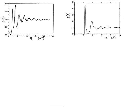
In the previous chapter we saw that in crystalline materials sharp di raction peaks appear at vectors K = G that satisfy the Bragg condition. This is not the case in noncrystalline solids. When the atomic positions are randomly distributed, rays scattered by di erent atoms interfere destructively because of the random phase di erence, so S(K) = 1 for every K except K = 0. Consequently g(r) = 1, that is, the pair-correlation function is identically zero. In amorphous materials, where short-range order is present, S(K) is not constant. Since amorphous samples are isotropic, spatial variations of the pair distribution function – i.e., the radial distribution function – can be determined from the variations of the elastically scattered beam using (2.1.24). Figure 10.2 shows the structure factor measured by neutron di raction and the derived radial distribution function for amorphous silicon.

Fig. 10.2. Structure factor of amorphous silicon measured by neutron di raction, and the derived radial distribution function. [S. Kugler et al., Phys. Rev. B 48, 7685 (1993)]

Smeared-out peaks in the structure factor may be interpreted as the broadened counterparts of the sharp Bragg peaks observed in crystals. This occurs because only short-ranged order is present and correlations exist only among first, second, and perhaps third neighbors. This closely parallels the situation in liquids, as discussed in Chapter 2.

For multicomponent amorphous materials di raction measurements reveal not only the total distribution function but also the so-called partial distribution functions. Consider, for example, a two-component system made up of NA atoms of type A and NB atoms of type B, both distributed randomly. The concentrations are

ci =	Ni	i = A, B .	(10.1.4)
	NA + NB

10.1 The Structure of Amorphous Materials

307

If scattering amplitudes are denoted by fA and fB and atomic positions by RAm and RBn then the amplitude of the scattered beam in the direction specified by the scattering vector K = k − k is the weighted sum of the amplitudes of the rays scattered by individual atoms. The intensity is therefore

I(K) = I f e−iK·RAm

0 A

m

Now we introduce the quantities

+	n	fBe−iK·RnB		2	(10.1.5)
				.

Γij (r) = N	Ni Nj	+ Rnj )2	,	(10.1.6)
	1 m=1 n=1 δ(r − Rmi
1

where N is the total number of atoms. Their Fourier transforms appear in the intensity

I(K) = I0N Γ (K) ,

(10.1.7)

where, if the scattering amplitudes are chosen real,

Γ (K) = f 2	Γ	(K) + f 2	Γ	(K) + 2f	f	B	Γ	AB	(K) .	(10.1.8)
A	AA	B	BB		A

The contribution K = 0 of forward scattering is customarily separated o from Γij (K); the remaining part defines the partial structure factor Sij (K)

	Γij (K) = cicj N δK,0 + cicj Sij (K) .			(10.1.9)
Substituting this into (10.1.8),
Γ (K) = N δK,0	f 2 c2	+ f 2 cB2 + 2fAfBcAcB
2 2	A A	B 2 2		(10.1.10)
+ fAcASAA(K) + fBcBSBB(K) + 2fAfBcAcBSAB(K) .

Direct scattering is seen to be proportional to (fAcA + fBcB)2 – as if the medium were monatomic, with an averaged scattering amplitude.

Partial structure factors are related to partial pair-correlation functions. Similarly to (2.1.1), up to a normalization factor gij (r) is defined as the probability for finding an atom of the jth type in an elementary volume dr around the point r when an atom of the ith type is located at the origin:

gij (r) = NiNj		Ni Nj	+ Rnj )2.	(10.1.11)
		1 m=1 n=1 δ(r − Rmi
	V

In the expressions for gAA and gBB the terms m = n are excluded. Along the same lines as in Chapter 2 it can be shown that

Γij (r) = δij ci δ(r) + ncicj gij (r) ,

(10.1.12)

308 10 The Structure of Noncrystalline Solids

where n = N/V ; in terms of the Fourier transforms

Γij (K) = δij ci + ncicj gij (K) .

(10.1.13)

Comparing this form with (10.1.9), making use of (2.1.20), and taking into account that amorphous materials are isotropic, one obtains

Sij (K) = δij ci			+ V		∞	4πr2 [gij (r) − 1]		Kr dr ,		(10.1.14)
					0
1				N				sin Kr
and
gij (r) = 1 + 8π3N			∞				Sij (K) − δij ci		Kr dK ,	(10.1.15)
			0	4πK2
	V						1		sin Kr

which are the generalizations of (2.1.23) and (2.1.24).

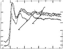
In neutron scattering the scattering amplitudes depend strongly on which particular isotope is used. Performing di raction measurements for various isotopic compositions, the partial structure factors, and from them the partial radial distribution functions may be determined. Such a set of experimental results is shown in Fig. 10.3.

S(K)

9

8

7

6

5

4

3

2

1

0

0

nat

Ni80P20 5

60

Ni80P20 2,5

62

Ni80P20

50 100 150

K (nm 1)

	14
	12
	10
)	8
(K
ij
S	6
	4

2

0

0

Ni Ni

P P 5

Ni P

50

100

150

K (nm 1)

Fig. 10.3. Structure factors measured for various isotopic compositions of a twocomponent amorphous material, Ni80P20 , and the derived partial structure factors. For better visibility, curves are shifted vertically. [P. Lamparter and S. Steeb, Proc. of the Fifth Int. Conf. on Rapidly Quenched Metals, p. 459 (1984)]

Besides the structure factors measured for three di erent isotopic compositions, the figure also shows the partial structure factors derived from

10.2 Quasiperiodic Structures

309

them. Their Fourier transform yields the pair-correlation functions shown in Fig. 10.4, more precisely the quantities

Gij (r) = 4πr[gij (r) − 1] .

(10.1.16)

As the figure shows, nearest neighbor Ni–Ni and Ni–P distances are practically equal, while nearest-neighbor P–P distances are larger than these. The arrangement of the two kinds of atom is therefore not perfectly random. Shortrange order appears because phosphorus atoms are preferentially surrounded by nickel atoms.

)2 nm

2 (10

( r)

ij G

40
35		Ni Ni
30
25
20		P P
15
10
5		Ni P
0
-5
0	0.5	1.0
	r	(nm)

Fig. 10.4. Partial distribution functions in amorphous Ni80P20. [P. Lamparter and S. Steeb, Proc. of the Fifth Int. Conf. on Rapidly Quenched Metals, p. 459 (1984)]

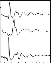
An e cient method for determining the local environment in disordered systems is EXAFS spectroscopy as the fine structure of the absorption edge is due to the interference of rays scattered by nearest neighbors. Figure 10.5 shows that the EXAFS spectrum of amorphous GeO2 has the same fine structure as GeO2 in its hexagonal crystalline form, and both are strikingly di erent from the spectrum observed in samples of tetragonal symmetry. This leads to the conclusion that locally, on atomic scales the arrangement of atoms in the amorphous state is very similar to that in the hexagonal crystalline phase.

10.2 Quasiperiodic Structures

In contrast to perfectly periodic order in crystals, amorphous materials may exhibit short-range order at best. In the past decades it has been revealed that nature o ers a wider variety of solid structures than that presented in the

310 10 The Structure of Noncrystalline Solids

coefficient										GeO2 (glass)
	yunits)								GeO2 (hexagonal)
sorption	arb(itrar
								GeO2	(tetragonal)
Ab
				0				100	200	300

Energy (eV)

Fig. 10.5. Fine structure of the absorption edge in amorphous and crystalline GeO2. [W. F. Nelson et al., Phys. Rev. 127, 2025 (1962)]

foregoing. There exist materials that do not possess discrete translation symmetries but nonetheless exhibit long-range order of some kind. Before turning to the investigation of such physical systems, some mathematical remarks are due.

10.2.1 Periodic and Quasiperiodic Functions

In Section 8.1 on the theory of di raction we saw that in systems composed of identical atoms the amplitude of the scattered beam is proportional to the structure factor, which is related to the Fourier transform of the spatial distribution of scatterers. Below we shall examine the di erences from this viewpoint between periodic, aperiodic (nonperiodic), almost periodic, and quasiperiodic functions. We shall use single-variable functions, however the obtained results are straightforward to generalize to the case of three spatial dimensions.

If a function f (x) is periodic with a period L – that is, f (x + L) = f (x) for all values of x – then it can be expanded in a Fourier series as

	∞
f (x) =	fne2πinx/L,	(10.2.1)

n=−∞

where n is an integer and

fn = L	L/2	e−2πinx/Lf (x) dx .	(10.2.2)
1

−L/2

The Fourier spectrum of a periodic function is therefore discrete. This corresponds to a sequence of equidistant Bragg peaks in the di raction pattern of a one-dimensional chain.

10.2 Quasiperiodic Structures

311

Changing to the variable k = 2πn/L and taking the limit L → ∞ opens the way to representing any nonperiodic function by a Fourier integral:

f (x) = 2π			∞	fˆ(k)eikx dk ,	(10.2.3)
		1
			−∞
where		∞
fˆ(k) =			f (x)e−ikx dx .		(10.2.4)

−∞

In this case the Fourier spectrum is continuous. This is typical of disordered systems.

There are, however, nonperiodic functions whose Fourier spectrum is discrete. Suppose that the Fourier transform of f (x) takes finite values on an infinite sequence λn of real numbers, that is its Fourier representation may be written as

f (x) =		ˆ	(10.2.5)
		f (λn) exp(2πiλnx) .

n

Such a function is called almost periodic: although it is not perfectly periodic in space, for every ε there exists a finite distance t such that

|f (x + t) − f (x)| ≤ ε

(10.2.6)

for all values of x.

Quasiperiodic functions constitute a special class of almost periodic functions. A function is called quasiperiodic if the infinitely many λn of its spectrum can be written as integer linear combinations of a finite number of irrational numbers αl (l = 1, 2, . . . , N ):

N
λn = nlαl ,	(10.2.7)
l=1

and the coe cients nl can take any integer values. In what follows, the label n will continue to refer to the set of coe cients n1, n2, . . . , nN . Using this notation, the Fourier representation reads

f (x) = n1

∞

n2

∞

∞

fn exp

N

αlnl

x

. (10.2.8)

=

=

. . . nN =

2πi l=1

−∞

−∞

−∞

Next we shall show that this function can be obtained from a function in N variables that is perfectly periodic in N -dimensional space when the values x1, x2, . . . , xN lie along a line. Consider the periodic function

F (x1

, x2

, . . . , xN ) = n1

∞

n2

∞

∞

fn exp

N

=

=

. . . nN =

2πi l=1 nlxl

−∞

−∞

−∞

(10.2.9)

312 10 The Structure of Noncrystalline Solids

defined in N -space. The quasiperiodic function f (x) can be obtained by restricting the previous expression to the line

x1 = α1x, x2 = α2x, . . . , xN = αN x ,	(10.2.10)
that is,
f (x) = F (α1x, α2x, . . . , αN x) .	(10.2.11)

Generalization of the above formulation to functions defined in threedimensional space is straightforward. It has already been mentioned that if a function f (r) is periodic in the lattice generated by the primitive translation vectors a1, a2, a3 then its Fourier series contains only components associated with vectors

3
k = G = hibi	(10.2.12)

i=1

of the reciprocal lattice, where the bi are the primitive vectors of the reciprocal lattice and the hi are integers. A function defined in three-dimensional space is called quasiperiodic if the vectors k in its Fourier expansion can be expressed as the linear combinations of more than three reciprocal-space vectors qi with integer coe cients hi,

N
k = hiqi ,	(10.2.13)

i=1

while the vectors qi are irrational linear combinations of the three primitive vectors bi. Then the allowed k vectors fill the reciprocal space densely. Nevertheless, as we shall see, the amplitude is very small for most of them, and the di raction pattern is dominated by a few discrete peaks.

10.2.2 Incommensurate Structures

Up to this point we have always spoken of periodic or nonperiodic arrangements of atoms. However, in solids the system of electrons may exhibit a periodicity di erent from that of the atoms, with the new wavelength determined by the properties of the electron system. We shall see examples for this in Chapters 14 and 33. It may happen that the wavelength ratio of atomic and electronic periodicities is not a rational number; in such cases the system is said to have an incommensurate structure. Strictly speaking periodicity is lost as the structure never repeats itself precisely because of the incommensurability of the two periods, nonetheless there exists a long-range order as it is possible to predict atomic and electronic densities precisely for any point in space.

To determine what di raction pattern would be obtained from a material with such a structure we consider, for simplicity, a chain of atoms with a lattice constant a and suppose that the electron system shows static density variations of wavelength λ that are described by a periodic function g(x):