Fundamentals of the Physics of Solids / 11-Dynamics of Crystal Lattices

11

Dynamics of Crystal Lattices

The discussion of the structure of solids was based on the assumption that atoms or ions are rigidly fixed at their equilibrium positions. Within the framework of classical physics this may be valid in the ground state of the crystal. However, at finite temperatures atoms are displaced by thermal motion from their equilibrium positions. Without taking this into consideration, certain mechanical, elastic, and thermal properties of solids could not be properly accounted for. For example, barring the regime of low temperatures, the calculated specific heat is found to be much smaller than the observed value when the vibration of ions is ignored and only the contribution of electrons is retained. Similarly, neither thermal expansion nor melting can be explained in a model that assumes the crystal structure to be rigid – not to mention mechanical properties, which do not lend themselves to interpretation in terms of a rigid lattice. Besides, lattice dynamics modifies the electronic states as well, as we shall see in the Volume 2.

Making use of the vacancies and interstitials in the lattice, atoms may move far from their initial position. In this chapter we shall ignore this di usion and assume that atoms stay close to their equilibrium positions (which correspond to a crystalline order), and perform small-amplitude oscillations about it. Here we shall treat the problem classically; quantum e ects will be taken into account in the next chapter.

11.1 The Harmonic Approximation

In principle, the motion of the atoms in a lattice can be determined unambiguously if the potential felt by them is known. In insulators only pairwise interactions among the atoms (interatomic pair potentials) need to be considered. In metals the full interaction is the sum of the direct Coulomb potentials due to other ions and the potential due to highly mobile delocalized electrons that are not bound to any ion. The interaction Hamiltonian therefore depends on the coordinates of ions and mobile electrons alike. We shall demonstrate

332 11 Dynamics of Crystal Lattices

in Chapter 23 that, owing to the large mass di erence between ions and electrons, electrons follow ions practically without any delay, while ions feel only an average of the potential due to electrons. In what follows we shall therefore assume that the potential U felt by the ions depends only on the ionic coordinates, just like in insulators.

For completeness we shall consider a lattice with a basis of p atoms at positions r1, r2, . . . , rp relative to the primitive cell; the lattice vectors of the primitive cells are denoted by Rm. The equilibrium positions of the atoms are

r0(m, μ) = Rm + rμ , μ = 1, 2, . . . , p.

(11.1.1)

When atoms perform thermal motion about these positions, their instantaneous coordinates at time t are given by

r(m, μ, t) = Rm + rμ + u(m, μ, t) ,

(11.1.2)

where u(m, μ, t) is the instantaneous displacement of the μth atom in the primitive cell at Rm from its equilibrium position. From now on, we shall usually suppress the time variable.

Obviously, the potential U is a function of the true atomic positions, and therefore of the displacements u(m, μ). To obtain an easily tractable problem, further assumptions have to be made about the interactions between ions.

11.1.1 Second-Order Expansion of the Potential

When the di usion of atoms is ignored, their displacement from equilibrium can be assumed to be small as long as the temperature is low compared to the melting point. The potential is then expanded in powers of the displacements u(m, μ) as

	U ({r(m, μ)}) = U0 +
		Φαμ (m)uα(m, μ)
		m,μ,α			(11.1.3)
	+	1	Φμν (m, n)uα(m, μ)uβ (n, ν) + . . . ,
		2	αβ
		m,μ,α
		n,ν,β
	where
	Φαμ (m) =			∂U ({r(m, μ)})	,
				∂uα(m, μ)
					(11.1.4)
	Φμν	(m, n) =		∂2U ({r(m, μ)})		.
	αβ			∂uα(m, μ)∂uβ (n, ν)

The Greek indices α, β label Cartesian coordinates.

The ground-state energy U0 – which corresponds to the configuration in which every atom is in its equilibrium position – is essential for the calculation of the total energy of the solid but unimportant for the determination of the

11.1 The Harmonic Approximation

333

frequency spectrum of vibrations, which is why it will be ignored below. Since the potential attains its minimum at the equilibrium positions of the atoms, the coe cients Φμα(m) of the terms linear in the displacement vanish. The approximation in which only second-order terms are kept is called the harmonic approximation. Throughout this chapter we shall use this approximation, as a relatively good description of the thermal properties of solids can be based on it. Phenomena that cannot be interpreted in this framework are presented at the end of the next chapter. In this context the role of higher-order terms in the expansion is also discussed there.

The ab initio determination of the coe cients Φ in the expansion is very di cult, and requires highly time-consuming numerical calculations. Therefore these coe cients are often considered as phenomenological parameters whose values are obtained from fits to experimental data. We shall also adopt this approach. Nevertheless there exist completely general relations among the coe cients through which the number of fitting parameters can be reduced substantially. One such relation is the consequence of the definition of the coe cients. As they appear as the second partial derivatives of the energy,

Φμν	(m, n) = Φνμ	(n, m) .	(11.1.5)
αβ	βα

Further relations are obtained from the expression of the force on individual atoms. The force on the atom labeled (m, μ) is derived from the potential as

F (m, μ) = −		∂U		(11.1.6)
			.
		∂u(m, μ)
In the harmonic approximation
Fα(m, μ) = −	Φαβμν (m, n)uβ (n, ν) .			(11.1.7)
	n,ν,β

Suppose that each atom is displaced by u0, which corresponds to a homogeneous translation of the crystal. Since atoms are not displaced relative to each another, the crystal remains in equilibrium, and the force on each atom is zero; hence

	(m, n) = 0 .	(11.1.8)
Φμν
αβ
n,ν
From (11.1.5) it follows that
	(m, n) = 0 .	(11.1.9)
Φμν
αβ

m,μ

By making use of the two previous formulas it is straightforward to show that the second-order term in the expansion of the potential may be written in the equivalent form

−41 Φμναβ (m, n) [uα(m, μ) − uα(n, ν)] [uβ (m, μ) − uβ (n, ν)] . (11.1.10)

m,μ,α

n,ν,β

334 11 Dynamics of Crystal Lattices

Yet another set of connections may be obtained by exploiting the property that a rigid rotation of the entire crystal does not generate any internal forces either. Even more important is that in specific cases knowledge of the crystal symmetries may substantially simplify calculations or the evaluation of measurements, as the same symmetries are shown by the potential U and so the coe cients Φμναβ as well. This possibility is nonetheless ignored in the general treatment.

As it will prove to be highly important for the applications below, it should be noted that in ordered crystals the coe cients Φμναβ (m, n) depend only on Rm − Rn, the di erence of the lattice vectors Rm and Rn of the primitive cells. Denoting this by m − n,

Φαβμν (m, n) = Φαβμν (m − n) .

(11.1.11)

11.1.2 Expansion of the Energy for Pair Potentials

In many – but by no means all – cases it may be assumed that the interaction among ions can be written as the sum of pair potentials that depend only on the di erence of the position vectors of the two ions:

U = 21
	Upair (r(m, μ) − r(n, ν))
	m,μ
	n,ν
	(11.1.12)
= 21
	Upair (Rm + rμ + u(m, μ) − Rn − rν − u(n, ν)) .

m,μ

n,ν

Expansion around the equilibrium position is then performed, and once again terms are kept only up to second order:

U = 12 Upair(Rm + rμ − Rn − rν )

m,μ

n,ν

%		(11.1.13)
+ 21	Φαμν (m, n) [uα(m, μ) − uα(n, ν)]
m,μ,α
n,ν	%
+ 41	[uα(m, μ) − uα(n, ν)] Φαβμν (m, n) [uβ (m, μ) − uβ (n, ν)] ,

m,μ,α

n,ν,β

where Φ% may now be expressed in terms of the first and second partial derivatives of the pair potential. Using the concise notation u = u(m, μ) − u(n, ν), we have

μν	(m, n) =	∂Upair(m, μ; n, ν; u)
Φ			,
α		∂uα
%μν					(11.1.14)
	(m, n) =	∂2Upair(m, μ; n, ν; u)
Φ%αβ					.
		∂uα∂uβ

11.1 The Harmonic Approximation

335

The term linear in the atomic displacements vanishes again, as the sum of the pair potentials has its minimum at the equilibrium distance of the ions. Comparing the second-order term with the expression in (11.1.10),

μν	μν	(m, n) ,	(11.1.15)
Φαβ	(m, n) = −Φ%αβ

unless m = n and μ = ν. To determine the contribution of the term m = n, μ = ν, a consequence of the relation (11.1.8) has to be exploited:

μν		%		%
Φαβ	(m, n) = δmnδμν	Φαβ (m, n ) − Φαβ			(m, n) .	(11.1.16)

n ,ν

Forces are said to be central when the pair interaction depends only on the distance between the atoms:

Upair(m, μ; n, ν; u) = Upair(|Rm+rμ+u(m, μ)−Rn−rν −u(n, ν)|) . (11.1.17)

Expansion of the potential about the equilibrium distance r = |r| = |Rm + rμ − Rn − rν | gives

∂Upair(|r + u|)	=	∂Upair(|r + u|)		rα + uα	,	(11.1.18)
		∂|r + u|
∂uα				r

which implies

μν		1 ∂Upair(r)			+	∂2Upair(r)		1 ∂Upair(r)
Φαβ	(m−n) = δαβ r ∂r					∂r2	− r ∂r
%

rαrβ . (11.1.19) r2

The first derivatives of the individual pair potentials do not generally vanish at the equilibrium position: only the full potential has its minimum there, which is why the first derivative appears in the expression for Φ%. The previous formula clearly shows that apart from an isotropic term the direction of the displacement relative to the axis joining the atoms is important. Restoring forces act only when the relative displacement of the atoms has a nonvanishing projection along this axis. Displacements perpendicular to it give only secondorder corrections to the interatomic distance, and therefore do not contribute to the energy.

11.1.3 Equations Governing Lattice Vibrations

The classical motion of atoms is most easily described using the Hamiltonian equations of classical mechanics. The Hamiltonian is specified by expressing the kinetic and potential energies in terms of the displacements u(m, μ) and the conjugate momenta. Assuming that each primitive cell contains an atom of mass Mμ at the μth position, the kinetic energy due to atomic vibrations is

Tkin = 12 Mμu˙ 2(m, μ) . (11.1.20)

m,μ

[uα(m, μ) − uα(n, ν)] Φ%μν (m, n) [uβ (m, μ) − uβ (n, ν)] .

αβ

or in terms of the pair potentials as

336 11 Dynamics of Crystal Lattices

The potential energy shall either be written as
Uharm = 21 Φαβμν (m, n)uα(m, μ)uβ (n, ν) ,	(11.1.21)
m,μ,α
n,ν,β

Uharm = 14

m,μ,α

n,ν,β

(11.1.22) In classical mechanics the canonical momentum P conjugate to the dis-

placement u is derived from the Lagrangian L = Tkin − Uharm as

P (m, μ) =	∂L	.	(11.1.23)
	∂u˙ (m, μ)

The kinetic energy then takes the form

	P 2	(m, μ)			P 2	(m, μ)
Tkin =			=		α		.	(11.1.24)
m,μ	2Mμ			m,μ,α	2Mμ

From the classical Hamiltonian, which is the sum of the kinetic and potential energies – both expressed in terms of the canonical variables –,

H = Tkin + Uharm ,

the following equations of motion are derived:

u˙ α(m, μ) =

∂H

=

Pα(m, μ)

,

∂Pα(m, μ)

Mμ

P˙

(m, μ) =

∂H

=

Φμν

(m

n)u

(n, ν) ,

α

−∂uα(m, μ)

−

αβ

−

β

n,ν,β

or

%

˙

μν

Pα(m, μ) = −

Φαβ (m − n)[uβ (m, μ) − uβ (n, ν)] .

n,ν,β

(11.1.25)

(11.1.26)

(11.1.27)

Di erentiation of the equation for u leads to the well-known Newtonian equation

Mμu¨α(m, μ) = − Φαβμν (m − n)uβ (n, ν) ,	(11.1.28)
n,ν,β
or alternatively
Mμu¨α(m, μ) = − Φαβμν (m − n)[uβ (m, μ) − uβ (n, ν)] .	(11.1.29)
n,ν,β
%

Since the potential is assumed to be harmonic, the equations are identical to those of a mechanical mass–spring system, which is why the quantities

11.2 Vibrational Spectra of Simple Lattices

337

Φμναβ (m−n) are called spring constants or force constants. The resulting manyvariable system of coupled di erential equations is seemingly very complex, however when plausible assumptions are made about the spring constants, it turns out to be solvable in some cases. The obtained intuitive picture facilitates the interpretation of the quantum mechanical results.

11.2 Vibrational Spectra of Simple Lattices

By considering the classical crystal as a system built up of N p mass points, the vibrations of the lattice are determined from the coupled system of equations (11.1.28) and (11.1.29) in 3N p variables. We shall first deal with some simple cases where calculations are straightforward. It will be assumed that atoms are located along a line, making up a chain, and their displacements are also in the same direction. In the simplest case the chain is made up of a single kind of atom, and nearest-neighbor distances are all identical in the equilibrium configuration. This model is called the monatomic linear chain. In a second, somewhat more complicated situation the chain is made up of two kinds of atoms of unequal mass, located at alternate positions. A similar treatment is applied in the case when the chain contains identical atoms and their equilibrium separations alternate. This system is called a dimerized chain. After the determination of the vibrational modes in these models we shall turn to the study of the vibrational spectra of simple cubic lattices, and then to the general discussion of classical vibrations in three-dimensional lattices.

11.2.1 Vibrations of a Monatomic Linear Chain

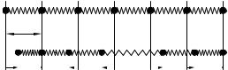
Consider a linear chain of lattice constant a with atoms of mass M at the lattice points. The origin of coordinates is chosen in such a way that the equilibrium position of the nth atom is na. The displacement un of each vibrating atom is supposed to be along the chain. The atoms, their equilibrium positions and displacements at time t are shown in Fig. 11.1.

n 1 n n 1

(a)

a

(b)

un 1 un				un 1

Fig. 11.1. Atomic positions in a one-dimensional monatomic chain (a) in equilibrium; (b) in vibration at an arbitrary time t. Springs represent the elastic forces between the atoms; un is the instantaneous displacement of the nth atom from its equilibrium position

338 11 Dynamics of Crystal Lattices

Using the form (11.1.13) for the harmonic potential,

U		= 1	%		u		]2
	harm	4		n −		n		(11.2.1)

nn

in this simple case. It is plausible to assume that the strength of the interaction decreases rapidly with increasing separation of the atoms, and so it is su cient to take into account only the e ects of the nearest neighbors. Denoting the spring (force) constant Φ%(n, n ± 1) by K,

Uharm = 21 K [un − un+1]2 .	(11.2.2)

n

The force on the atom is its derivative, i.e., the equation of motion for the nth atom is

M u¨n = −	∂Uharm	= −K [2un − un−1 − un+1] .	(11.2.3)
	∂un

The solution of the system of coupled di erential equations requires the specification of the boundary condition. A practical choice is the periodic or Born–von Kármán boundary condition, whereby the N atoms are assumed to be not along a free chain of length L = N a but on a ring of the same circumference, and so the N + 1st atom is the same as the first. Then

uN +1 = u1 .

(11.2.4)

As traveling waves are expected to propagate in the mass–spring system, the solution is most easily obtained using a Fourier expansion for the displacements. The discrete position variable is thus replaced by the discrete wave number q, and the continuous time variable by the continuous frequency

	variable ω:				∞
	un(t) = √N		q	2π		dω u(q, ω)ei(qna−ωt) .	(11.2.5)
	1			1
					−∞

Since displacements are real, the pairs (q, ω) and (−q, −ω) describe the same atomic vibration. Therefore we shall permit q but not ω to take negative values.

The periodic boundary condition allows only those values of q for which eiqN a = 1, that is

2π	, j = 0, ±1, ±2, . . . .
q = j N a		(11.2.6)

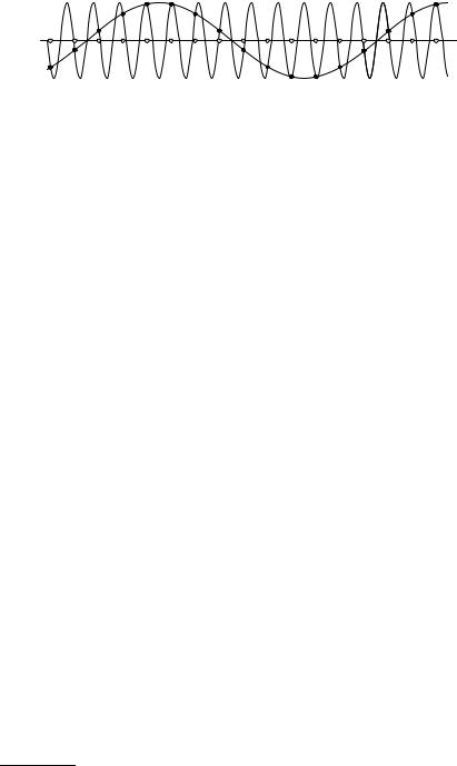
When two integers j di er by an integral multiple of N , the di erence of the corresponding wave numbers is an integral multiple of 2π/a. As illustrated in Fig. 11.2, such waves describe the same atomic displacement because un is defined only in discrete lattice points.

11.2 Vibrational Spectra of Simple Lattices

339

Fig. 11.2. Atomic displacements for the Fourier components with wave numbers q and q + j 2π/a. For transparency, displacements are shown perpendicular to the chain. The graphs of the waves drawn with solid and dashed lines have physical meaning only in discrete lattice points

In the description of lattice vibrations wave numbers that di er by 2π/a are thus equivalent. Since b = 2π/a is the primitive vector in the reciprocal lattice of a one-dimensional lattice, the previous assertion establishes the equivalence of wave vectors that di er by a reciprocal-lattice vector. This is in accordance with the general consequences of discrete translational symmetry discussed in Chapter 6. Once again, the N independent qs are customarily chosen in the Brillouin zone; for a one-dimensional chain this is the region

−π/a < q ≤ π/a .

(11.2.7)

The restriction on wave numbers can be interpreted in another way by asserting that it is meaningless to speak about oscillations whose half wavelength is smaller than the lattice constant. Therefore we shall always represent the spectrum of lattice vibrations inside the Brillouin zone.

Substituting the Fourier transform into the equation of motion (11.2.3), the Fourier components of di erent wave numbers do not mix. In the harmonic approximation waves of di erent wavelengths propagate independently. The equation for the Fourier component u(q, ω) is

−M ω2u(q, ω) = −K 2 − e−iqa − eiqa u(q, ω)

(11.2.8)

= −2K [1 − cos qa] u(q, ω) .

The angular frequency of the oscillation of wave number q is then

ω(q) =		2K(1 − cos qa)		= 2		K	1/2	sin	1 qa .
											(11.2.9)
/		M			M				2

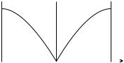
The relationship between the vibrational frequency1 and the wave number – the dispersion relation – is shown in Fig. 11.3.

In the long-wavelength limit (1/q a) the curve is linear:

ω(q) ≈	M		1/2	(11.2.10)
			a |q| .
		K

1The notation ω is always used for angular frequencies, however we shall follow common practice and use the term frequency instead of angular frequency.

340 11 Dynamics of Crystal Lattices

!(q)

		q
- /a	/a

Fig. 11.3. Dispersion curve for the longitudinal vibrations of a monatomic linear chain

In this limit neighboring atoms oscillate almost perfectly in phase, and the motion corresponds to the oscillation of an elastic continuum, i.e., the propagation of sound waves. For this reason such vibrations are called acoustic vibrations.

When lattice vibrations are combined into a wave packet, the group velocity is

∂ω(q)

K

1/2

qa

c =

∂q

=

M

a cos 2 .

(11.2.11)

Starting from the midpoint of the Brillouin zone the group velocity is monotonically decreasing. As shown in the figure, the dispersion curve has extrema at the boundaries of the Brillouin zone; it becomes flat there, so its derivative, the group velocity vanishes. This is the consequence of the reflection symmetry in monatomic linear chains.

It is straightforward to demonstrate that some characteristic features of the dispersion curve are preserved when not only first neighbors interact. Denoting the force constant of the interaction between pth neighbors by Kp, the potential is

Uharm = 21				Kp [un − un+p]2	(11.2.12)
				n,p
in the harmonic approximation, and so the equation of motion is
M u¨n =		Kp [2un − un+p − un−p] .			(11.2.13)
	p
Eigenfrequencies are then given by
	2
ω2(q) =				Kp [1 − cos(pqa)] .	(11.2.14)
		M
				p

It is readily seen that ω is always an even function of q,

ω(q) = ω(−q) .

(11.2.15)

This formula reflects the symmetry that waves can equally propagate to the left and to the right along the chain. This result is generally valid: as it was