Lect5-Optical_fibers_2

Limiting bit rate near zero-dispersion wavelength

•  Now it becomes clear that at λ = λZD, the dispersion slope So becomes the bit rate limiting factor. We can estimate the limiting bit rate by noting that for a source of spectral width Δλ, the effective value of dispersion parameter becomes

	D = So Δλ
=>	The limiting bit rate-distance product can be given as
	BL |So| (Δλ)2 < 1	(B T < 1)

*For a multimode semiconductor laser with Δλ = 2 nm and a dispersionshifted fiber with So = 0.05 ps/(km-nm2) at λ = 1.55 µm, the BL product approaches 5 (Tb/s)-km. Further improvement is possible by using

single-mode semiconductor lasers.

111

Dispersion tailored fibers

1.  Since the waveguide contribution Dwg depends on the fiber parameters such as the core radius a and the index difference , it is possible to design the fiber such that λZD is shifted into the neighborhood of 1.55 µm. Such fibers are called dispersion-shifted fibers.

2. It is also possible to tailor the waveguide contribution such that the total dispersion D is relatively small over a wide wavelength range extending from 1.3 to 1.6 µm. Such fibers are called dispersionflattened fibers.

112

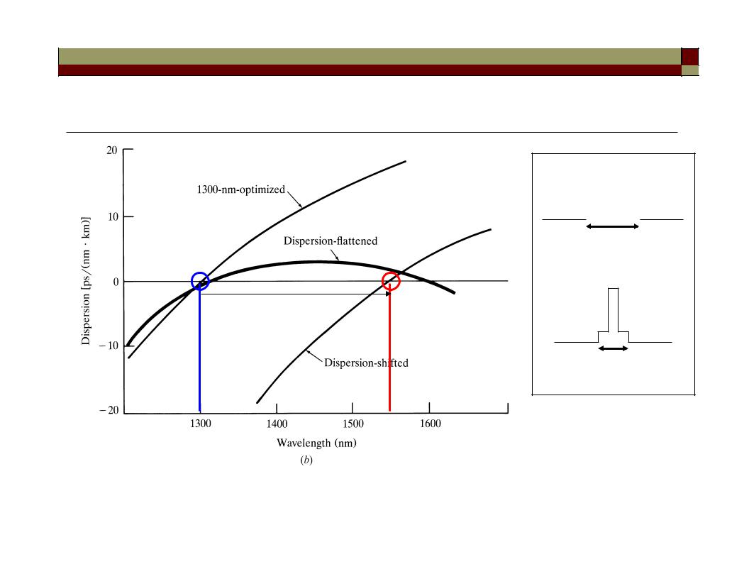
Dispersion-shifted and flattened fibers

(standard) ncore(r)

ncore(r)

•  The design of dispersion-modified fibers often involves the use of multiple cladding layers and a tailoring of the refractive index profile.

113

Non-zero dispersion shifted fibers

•  Since dispersion slope S > 0 for singlemode fibers => different

wavelength-division multiplexed (WDM) channels have different

dispersion values.

km]

*SM fiber or non-zero

[ps/nm-

dispersion-shifted

fiber (NZDSF) with

D ~ few ps/(km-nm)

Dispersion

WDM

λ

1500

1550

1600

*In fact, for WDM systems, small amount of chromatic dispersion
is desirable in order to prevent the impairment of fiber nonlinearity
(i.e. power-dependent interaction between wavelength channels.)	114

Chromatic Dispersion Compensation

•  Chromatic dispersion is time independent in a passive optical linkallow  compensation along the entire fiber span

(Note that recent developments focus on reconfigurable optical links, which makes chromatic dispersion time dependent!)

Two basic techniques: (1) dispersion-compensating fiber DCF

(2) dispersion-compensating fiber grating

•  The basic idea for DCF: the positive dispersion in a conventional fiber (say ~ 17 ps/(km-nm) in the 1550 nm window) can be compensated for by inserting a fiber with negative dispersion (i.e. with large -ve Dwg).

115

Chromatic dispersion accumulates linearly over distance

(recall	T	=	D L Δλ )
(ps/nm)
dispersion			time
			+D (red goes
			slower)
Accumulated			Positive dispersion
			transmission fiber
			time

Distance (km)	116

Chromatic Dispersion Compensation

Positive dispersion transmission	Negative dispersion element
fiber

(ps/nm)		-D’		-D’		-D’
Accumulated dispersion	+D	-D’	+D	-D’	+D	-D’
						Distance (km)

•  In a dispersion-managed system, positive dispersion transmission
fiber alternates with negative dispersion compensation elements,
such that the total dispersion is zero end-to-end.	117

Fixed (passive) dispersion compensation

Dispersion [ps/nm-km]

SM

+ve

			17	+ve
SM fiber						λ
			λο
	DCF		-80	-ve (due to large -ve Dwg)
DCF	SM		DCF	SM		DCF
-ve	+ve		-ve	+ve		-ve

*DCF is a length of fiber producing -ve dispersion four to five times
as large as that produced by conventional SMF.	118

Dispersion-Compensating Fiber

The concept: using a span of fiber to compress an initially chirped pulse.

Pulse broadening with chirping

Pulse compression with dechirping

λl

λs

λl

λs

λs

λs

λl

λl

Initial chirp and broadening by a transmission link

Compress the pulse to initial width

L1

L2

Dispersion compensated channel: D2 L2 = - D1 L1

119

Dispersion-Compensating Fiber

			Conventional fiber (D > 0)		DCF (D < 0)
	Laser					Detector
			L		LDCF

e.g. What DCF is needed in order to compensate for dispersion in a conventional single-mode fiber link of 100 km?

Suppose we are using Corning SMF-28 fiber,

=>	the dispersion parameter D(1550 nm) ~ 17 ps/(km-nm)
	Pulse broadening Tchrom = D(λ) Δλ L ~ 17 x 1 x 100 = 1700 ps.

assume the semiconductor (diode) laser linewidth Δλ ~ 1 nm.

120