Лекции_Микроэкономика

A.Friedman

ICEF-2012

$	MB
		MC
	c	care, c

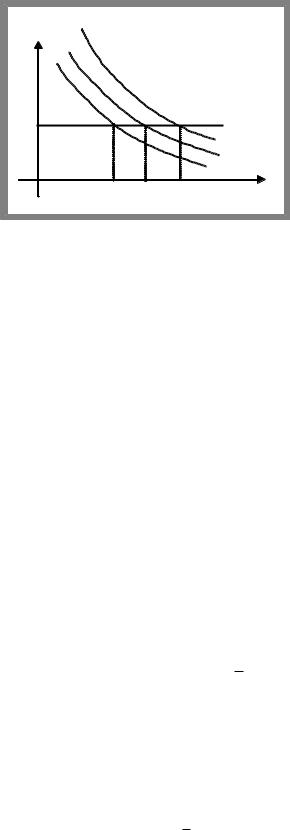
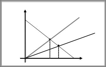
Now, suppose this person buys full insurance at fair price based on efficient level of care. Then his MB curve shifts down since losses in case of fire will be covered by insurance company. As a result the level of care taken by the person goes down. The less care is taken, the greater is the probability of accident, which increases the chance that insurance company will have to pay. Thus there is a moral hazard problem.

Outcome is inefficient since the level of care is smaller than efficient.

$
MBinsuranceMB
	DWL
		MC
cins	c	care, c

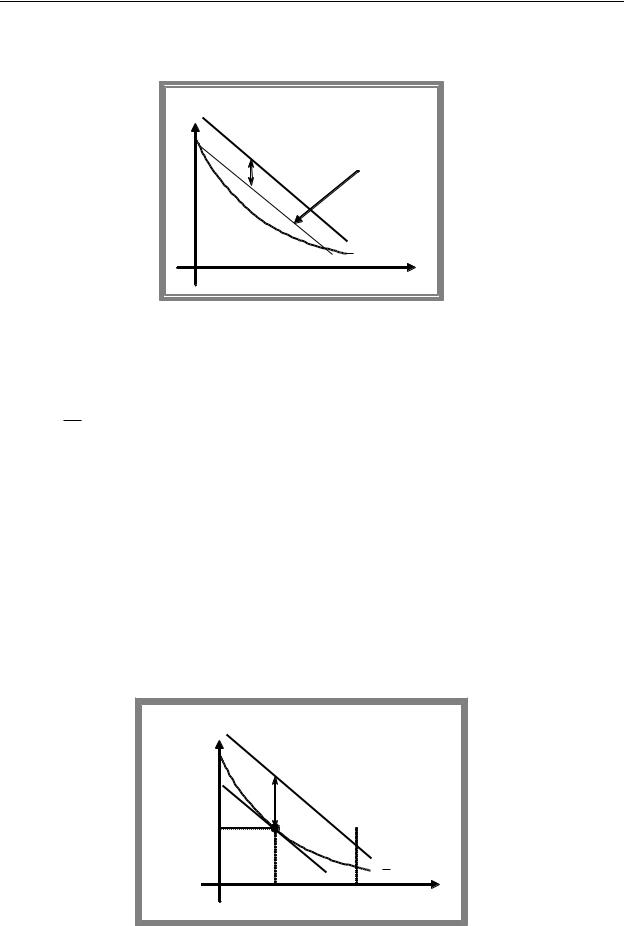
Since level of care taken is smaller than efficient and expected losses goes up this is reflected in higher insurance premium.

The problem comes from non-observability of the level of care. Had the level of care be observable, insurance rates could be set as a function of the level of care: low level of care could be accomplished by high insurance rates and high level of care with low rates.

But if care is not observable, than every potential policyholder finds optimal to promise high level of care to get low insurance premium. Insurance companies understand the problem and as a result expect low level of care if care is not observable and only high insurance premiums are offered at the market.

Responses to moral hazard problem.

The problem of moral hazard arises because insurance reduces the incentives for care. One way to solve the problem is to reduce the level of insurance and require the policyholder to bear some of the costs of claim.

This cost sharing generally takes one of two forms:co-insurance,

111

A.Friedman

ICEF-2012

deductibles.

In case of co-insurance insurance company pays for less than 100% of the bill and the policyholder picks up the rest.

Under a deductible the person buying the insurance has to pay the initial damages up to some set limit.

$	MB
			MC
			MBco ins
		MB full ins
	cins cco ins	ceff	care, c

Both polices are unable to solve the problem completely. On one hand some moral hazard remains as long as some insurance is provided as private marginal benefit is below the social one. On the other hand under both policies insurance is not full, which indicates inefficient allocation of risk.

9.4 Moral hazard in labour markets

The principal-agent model gives another example of moral hazard problem.

Agent is hired by principle to perform certain tasks. Moral hazard problem arises when principle and agent have different goals and actions of agent can’t be monitored by principle. As a result agents may take actions that are not in the interests of the principle.

Assumptions of the model

owner of the firm maximizes profit and hires manager to run the firm,

owner’s gross profit is diminishing in shirking hours s : s , s 0 ;

	owner behaves like monopsonist, he offers a contract that specifies s, y and manager
	can accept or reject the offer,
	manager maximizes his utility, which is increasing in aggregate commodity and in
	shirking hours: u s, y , where u s, y 0	and u s, y 0 , s 0,T ;
	s	y

price of aggregate commodity is normalized and equals 1,

alternative employment gives manager utility level of u .

Equilibrium under observable shirking

If the shirking is observable, then the optimal contract is given by the combination of salary

( y ) and shirking time ( s ) that maximise the net profit of the firm’s owner: max s y

	y ,s	.
	s.t. u s, y u
		112

A.Friedman

ICEF-2012

Note that optimal contract brings exactly reservation utility (otherwise by decreasing y we can still satisfy the constraint but increase the net profit).

Optimal contract brings maximum to the Lagrangean: L s, y, s y u s, y u .

		s u			u	s .
			s	or MRS
	FOCs:				s
		1	u y		u y
				sy

Thus optimal contract corresponds to a tangency point of reservation indifference curve with profit curve.

y
net
profit
y		s
		u
s	T	s

Unobservable shirking

If shirking is unobservable, then compensation can not be based on the amount manager shirks.

(i) In this case owner may offer flat salary scheme, where compensation is constant. As utility of manager is increasing in shirking and compensation does not depend on the amount he shirks finds optimal to shirk all the time, i.e. s flat T . The optimal level of salary is the one that is the lowest possible that attracts the manager (if it is profitable at all), i.e. y flat is the

solution of the equation u T , y flat u .

y
	s	net
y flat	u	profit
s	T	s

As agent will shirk all the time, shirking is not at efficient level. TS is reduced as under the same utility of manager the net profit of owner is reduced.

(ii) To get efficient solution owner should provide incentives for effort to emerge. This can be done via performance based compensation. If owner ties the manager’s payment to the profitability of the firm, manager will care about shirking hours since it directly affects the

113

A.Friedman ICEF-2012

profit, which determines his compensation. Suppose that firms owner gets some fixed sumG of money and the residual profit s G goes to the manager so that he becomes a residual claimant.

			y
				G	s G
					s
					u
					s
Then manager for any given value of				G solves the following problem: max u s, s G .
						s 0,T
Solving this problem, we get a best response function of manager						s G . For interior case
s G		is	given by the solution of	equation u s, s G u		s, s G s 0	or
				s	y
MRS			u
	sy		s s . As usually consumer chooses a point of tangency of budget line with
			u y

indifference curve.

Note that G stays for the profit of the owner, thus he wants to maximise G taken into account that the resulting utility level of the manager has to be equal or above the value of reservation utility:

max G

G		.
s.t. u s G , s G G
	u

Thus owner has no incentive to overcompensate the manager and will choose the level of G that gives exactly the reservation utility level. Thus optimal contract lies on reservation indifference curve and is characterised by a tangency of indifference curve with budget line (residual profit line), i.e. the contract corresponds to the same level of effort as the one under observable efforts.

y

G

s G		s
	s G	u
s	T	s

Conclusion: residual claimant compensation scheme is superior to flat salaries.

114

A.Friedman

ICEF-2012

But residual claimant scheme solves the problem of moral hazard only in case, when manager is risk neutral. However, if manager is risk averse, then this is not the case. Note that residual claimant bears all the risk associated with the business. There is no sharing of risk with the owner, which is optimal under observable efforts given that owners are risk neutral. Thus with unobservable efforts we face a trade-off between providing incentives and risk sharing.

115

A.Friedman

ICEF-2012

10. EXTERNALITIES, PUBLIC GOODS AND PUBLIC CHOICE

An externality refers to the effect when one economic agent’s action directly confers benefit or imposes a cost on some other agent without that consequence being reflected directly in market prices and exchange transactions.

Externalities can be positive or negative.

A positive externality occurs when one economic agent creates a benefit for another (without compensation).

A negative externality occurs when one economic agent imposes a cost on another (without compensation).

Externalities can be divided into 4 categories according to the source-recipient principle:

Consumption-consumption (smoker sitting next to a table of non-smokers in a restaurant),

Consumption-production (healthy lifestyle increases productivity),

Production-consumption (factory pollutes the air in the area where people live),

Production-production (factory pollutes the water used by another firm).

10.1 Externalities as a source of market failure

Externalities can adversely affect economic efficiency as complete market system assumption or the assumptions of the FFWT is not satisfied, i.e. externalities results in missing market problem.

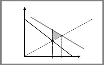
Inefficiency in case of externalities arises due to difference between social marginal benefit (SMB) and private marginal benefit (PMB) and/or social marginal cost (SMC) and private marginal cost (PMC). Let’s illustrate this point by an example of a positive externality in consumption. In this case SMB>PMB, while PMC=SMC.

P,MC

PMC=SMC

A

B	SMB
C	PMB
Qeq Qeff	Q

By moving from Qeq to Qeff gross CS increases by area A+B+C, while costs rises only by B+C, so TS increases by A. It means that equilibrium is inefficient, in particular, there is underproduction of Q as agents do not take into account the positive external benefit from consumption. As a result at equilibrium we have DWL= TS=A.

In case of negative externality there will be underproduction in equilibrium (since PMB>SMB if we deal with consumption externality) which is also associated with DWL.

Efficient output is determined by equality of social marginal benefit and social marginal cost. If each unit of good X produced imposes external damage, we should differentiate between

116

A.Friedman ICEF-2012

social and private marginal costs. Social marginal cost can be calculated as a sum of private marginal cost and marginal damage: SMC( Q ) PMC( Q ) MD( Q ) . Equating SMB and SMC, we get the efficient level of output.

P,MC

SMC

P(Q)

PMC

A
B
C
Qeff Qeq	Q

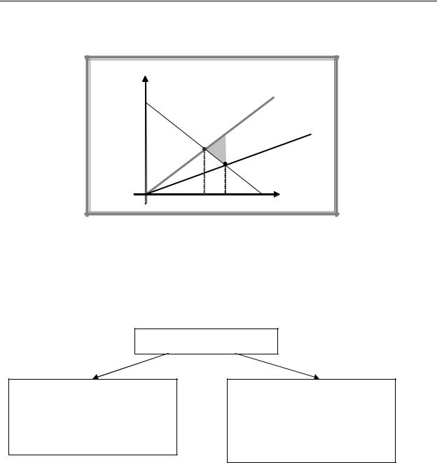
Green triangle illustrates DWL resulting from negative externality. If output increases from Qeff to Qeq , then total benefit goes up by area (B+C), while social cost rises (A+B+C). As

cost increases more than benefit, total surplus is reduced by area of A, corresponding to dead weight loss.

10.2 Responses to externalities

Responses to externalities

Private responses

Internalization via mergers

Social conventions

Bargaining (Coase theorem)

Government responses

Direct regulation

Corrective taxes

Creating a market (marketable pollution permits)

Private responses

Internalization.

An externality can be internalized by combining the involved parties, i.e. putting the problem in the hands of a single decision maker.

If firm A pollutes the water while firm B suffers from pollution, then the combined firm (if merging takes place) will take into account the negative impact of water pollution as it would maximize the total profit.

Social conventions.

Individuals cannot merge in order to internalize the externalities. Instead social conventions are used to force people to take into account the externalities they generate.

Bargaining and the Coase theorem.

117

A.Friedman

ICEF-2012

Suppose that property rights are assigned. Then parties may bargain and if bargaining is costless then they will reach the mutually beneficial solution.

Let us take the case of permissive law, when polluting firm has legal right to pollute. Assignment of property rights allows determining the default option (disagreement point). If firm pollutes the air and consumers suffer from pollution, then equilibrium level of pollution

Q 0 will take place without agreement.

But consumers are willing to pay firm to reduce pollution. The maximum compensation offered equals the value of marginal damage. Firm is willing to produce less (and reduce pollution) if compensation is at least equal to the profit forgone. As marginal profit is less

than MD for any Q Q , then in the absence of transaction costs output will be reduced up to

Q .

$

SMC

P(Q)

PMC

0	Q	Q0	Q

Now let us take the restrictive law case, where consumers have legal right for clean air. Now disagreement point corresponds to zero output.

In this case firms are willing to pay consumers to be able to produce and consumers are willing to increase pollution only if they are compensated for the marginal damage. Thus as far as compensation proposed (maximum compensation corresponds to the value of marginal profit) exceeds the minimum compensation required (equal to the value of MD), the output

will go up. As marginal profit exceeds MD for any Q Q , then in the absence of transaction costs output will be increased up to Q .

Thus we arrive at the essence of the Coase theorem: private negotiations will result in an efficient solution independently of who is assigned the property rights, as long as the initial legal assignment of rights is well defined and transactions involving exchange of rights are costless.

Reasons for failure of negotiations

Property rights (if property rights are not well assigned, then there is uncertainty about default option which prevents parties from reaching the mutually beneficial agreement).

Cost of bargaining (if bargaining is not costless, then parties would be unable to reduce pollution below the level where marginal profit equals to MD + bargaining cost.)

Difficulty in identifying source of damages (Even if ownership rights for clean air were established, it is not clear how the owners would be able to identify which of the thousands of potential polluters were responsible for dirtying their air space).

118

A.Friedman

ICEF-2012

Free-rider problem. If we assume that firms have the right to pollute the air and there is a large number of air pollution recipients it is unlikely that recipients will be able to agree among themselves on their respective contributions to a fee that would induce the firms to reduce pollution to an efficient level. Each recipient will have an incentive to understate his willingness to contribute (assuming that contribution of others will give the desired level of pollution). But if everybody behaves in such a way the total contribution will fall below the amount required to compensate the firms and the air would be dirtier than optimal.

Suppose we have 2 players (A and B). Each one can make a contribution or not. If both contribute, then pollution is reduced to efficient level and each agent gets net benefit of $15. If only one contributes and the other does not, then pollution is reduced but still exceeds the efficient level. The contributor’s net benefit equals -$10, while the benefit of the other person is $20. If nobody makes the contribution, then both suffer from pollution and net benefit of each player equals -$5.

	Player B
	Free ride	Contribute
Player A Free ride	-5, -5	20, -10
Contribute	-10, 20	15, 15

As -5>-10 and 20>15, free ride is a dominant strategy for each agent. As a result nobody contributes and each suffers from excessive pollution in equilibrium. Outcome is inefficient as by contributing both would be better off.

Hold-out problem. If recipients have legal right to clean air and are compensated by the polluting firm, then each has an incentive to overstate the compensation required. As a result of hold out problem they are unable to agree on the size of compensation.

Small numbers bargaining problem in presence of asymmetric information. Suppose there are only two agents involved. Let us assume that the minimum compensation required to allow pollution is $10, while benefit from pollution is $15, which implies that mutually beneficial agreement could be achieved if transaction costs are zero. Suppose that information on values of marginal damage and marginal profit is private and is not known by the other side. If the party that offers compensation (firm) thinks that the value of damage is $8 and offers a payment of $9 then this offer is rejected, but then firm thinks that the other side is simply bluffing and breaks off negotiations.

Government responses

Direct regulation

To correct negative externalities government can impose the maximum limit on pollution (that corresponds to efficient level) or require installing special equipment that reduces pollution.

To correct positive externality government can introduce the minimum requirement on the level of output.

Problems. To make direct regulation efficient government needs private information on costs of production, which is problematic.

Corrective tax

119

A.Friedman

ICEF-2012

Inefficiency can be eliminated if per unit tax (in case of negative externality) or subsidy (in case of negative externality) is introduced. This tax/subsidy is called Pigouvian tax.

This per unit tax/subsidy should be equal to the value of MEC (or MEB) evaluated at the efficient level of output. Figure below illustrates how the Pigouvian tax works. It shifts the supply function upward exactly by the value of tax and, as a result, equilibrium output falls.

Information: SMB and SMC to calculate Qeff as a point of intersection of SMB and SMC; PMB to find the value of corrective tax rate t=SMC(Qeff)-PMC(Qeff)= MD(Qeff).

P,MC

SMC

P(Q)

PMC+t

PMC

t

Qeff	Q

Creating a market (marketable pollution permits)

A fixed total number of permits is issued (efficient one) and each firm is allowed to pollute no more that the amounts stated on the permits it holds. Firm may change the quantity of permits by selling or buying permits at free market. Any polluter that generates emissions in excess of permits is subject to substantial monetary sanctions.

Comparison of government responses

	Direct regulation	Tax	Marketable pollution
			permits
Level of pollution	Certain	uncertain	certain
Additional revenues	No	yes	yes if auctioned
Cost minimization in	No	yes	Yes
reduction of pollution
Automatic instrument	No need	No	Yes
adjustment to inflation
Other comments			Might be used as an
			instrument of entry
			deterrence

In presence of different producers responsible for pollution, if information about the type of producer is asymmetric, direct regulation usually requires equal reduction of pollution by all firms. But equal reduction under heterogeneity of firms is not necessarily a cost minimising way of reduction of pollution.

Example. 2 firms with different marginal abatement costs. As can be seen from the graph uniform regulation results in higher total abatement cost that uniform tax.

120