1greenacre_m_primicerio_r_multivariate_analysis_of_ecological

Exhibit 11.1:

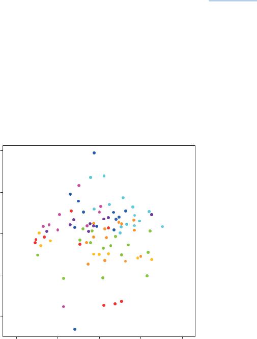
Locations of samples in “Barents fish” data set. At each sampling point the data consist of the abundances of 30 fish species, the bottom depth, the temperature and the spatial position (latitude

and longitude). The stations have been colour coded into approximately neighbouring groups, using great circle distances, for comparison with the MDS map based on the abundances (coming in Exhibit 11.3)

MULTIVARIATE ANALYSIS OF ECOLOGICAL DATA

Svalbard

Barents

Sea

Norway

Russia

and the latitude/longitude coordinates for each sample. A small part of the data set is shown in Exhibit 11.2, showing that the species abundances differ widely both among samples and among species (see the sums of the rows and columns shown). Nevertheless, the samples come from equal volume sampling, a 20-min- ute bottom trawl in each case.

	Exhibit 11.2:	STATION			ENVIRONMENTAL DATA								SPECIES ABUNDANCE DATA
	Part of the “Barents fish”
																				Sum
		ID No			Latitude	Longitude	Depth	Temp. Re_hi An_de An_mi					Hi_pl An_lu Me_ae Ra_ra				···	Ca_re Tr_spp
	data set: 89 samples (rows),
	4 environmental variables
		356			71.10	22.43	349	3.95	0		0	0	31	0	108	0	···	0	0	845
	and 30 fish species
		357			71.32	23.68	382	3.75	0		0	0	4	0	110	0	···	0	0	1,740
	(columns)
		358			71.60	24.90	294	3.45	0		0	0	27	0	788	0	···	0	0	1,763
		359			71.27	25.88	304	3.65	0		0	1	13	0	295	0	···	0	0	767
		363			71.52	28.12	384	3.35	0		0	0	23	0	13	2	···	0	0	1,347
		364			71.48	29.10	344	3.65	1		0	0	20	0	97	0	···	0	0	801
		·			·	·	·	·	·		·	·	·	·	·	·	·	·	·	á
		·			·	·	·	·	·		·	·	·	·	·	·	·	·	·	á
		·			·	·	·	·	·		·	·	·	·	·	·	·	·	·	á
		462			70.83	21.32	167	4.45	0		0	0	10	2	50	0	···	0	0	232
		465			73.38	17.37	462	1.95	0		0	0	0	0	0	0	···	0	0	36
								Sum	316		135	45	8,564	9	6,141 305		ááá	62	653	63,896

140

MULTIDIMENSIONAL SCALING BIPLOTS

In order to perform MDS on these data, either Bray-Curtis or chi-square can be computed, bearing in mind the differences between them when they are applied in their usual forms: Bray-Curtis is computed on the original abundances, whereas chi-square is applied to the relative abundances in each sample. There is also the issue about whether abundances should be transformed before applying Bray-Curtis, for example a square root or even fourth root transformation. We first compute Bray-Curtis on the raw data and then consider transformations later in this chapter. Exhibit 11.3 shows the nonmetric MDS solution in two dimensions of the Bray-Curtis dissimilarities, with the same colour coding as in the geographical map of Exhibit 11.1. The MDS solution is interpreted spatially as the similarity between the samples in terms of their species abundances, while Exhibit 11.1 represents the geographical proximities between the sampling locations. Already we can see in Exhibit 11.3 that points in the same spatial group (colour-coded) are often close together. So we can consider here the interesting question of measuring how similar the biologically determined map is to the geographical map. A simple approach

Relating MDS map to geography

1.0

0.5

2	0.0
Dimension
	–0.5

–1.0

–1.0

–0.5

0.0

0.5

1.0

Dimension 1

Exhibit 11.3:

Nonmetric MDS of the Bray-Curtis dissimilarities in community structure between the 89 samples, with the same colour coding as in the map of Exhibit 11.1

141

Exhibit 11.4:

Scatterplot of inter-sample geographical (great circle) distances and distances in Exhibit 11.3. Spearman rank correlation 0.378

MULTIVARIATE ANALYSIS OF ECOLOGICAL DATA

2.0

	1.5
NMDS distances	1.0

0.5

0.0

0

200

400

600

800

1,000

1,200

Great circle distances

is to plot the two sets of inter-sample distances against one another (there are ½ 89 88 3,916 of them), shown in Exhibit 11.4. The Spearman rank correlation between the two sets of distances, which measures how similar the two sets of distances are, is equal to 0.378.

An alternative approach is to use Procrustes analysis, a method that is specifically designed to measure the similarity between two maps. One of the maps, in this case the geographical map, is used as a target matrix and the other one, the MDS map, is rotated, translated and rescaled to best fit the target. One possible problem here is that the Euclidean distances between the latitude/longitude coordinates do not give the great circle distances. This can be solved by using a map projection in R (see Appendix C) to get coordinates for which Euclidean distances are approximate great circle distances. The Procrustes correlation between Exhibits 11.1 (using projected coordinates) and 11.3 turns out to be 0.549 and highly significant (p < 0.0001), hence there is a relationship between the geography and the fish community structure.

142

MULTIDIMENSIONAL SCALING BIPLOTS

As presented in Chapter 10, we use the regression biplot to add species and environmental variables to an MDS map such as Exhibit 11.3. A Poisson regression of every species can be performed on the two dimensions of the map, and the species depicted by the gradient vector of its regression coefficients. For every environmental variable (here we have two, but we can include latitude and longitude as well for the moment) a linear regression can be performed on the two dimensions of the map, again providing a gradient vector in each case. The result is shown as a separate display in Exhibit 11.5.

Notice several technical aspects of this display. First, each Poisson regression models the logarithm of the mean species abundance, so that biplot axes through the species vectors, if calibrated, would have logarithmic scales. On the other hand, the biplot axes indicated by the environmental variables would be calibrated linearly – see Chapter 10. Second, to equalize the scales of the environmental variables, they were standardized. Third, because of the dispar-

Adding continuous variables to a MDS map

	4						Ly_se
							Le_de
					Ly_pa	Ar_at
						Ly_re
	2
					LatHi_pl
			Ly_es	Ly_eu
	No_rk			Re_hi	Ra_ra	Ca_re
					An_de
					An_lu	An_mi Long
						Lu_la		Ga_mo
2						Ma_vi
	0					Be_gl
Dimension		Se_me	Depth
						Ly_va
				Cy_lu		Se_ma
						Le_ma
	–2				Temp Tr_spp
				Cl_ha
								Me_ae
				Bo_sa
	–4					Mi_po
								Tr_es
	–6	–4		–2	0	2		4

Dimension 1

Exhibit 11.5:

Gradient vectors of the species (from Poisson regressions) and of the environmental variables (from linear regressions) when regression is performed on the dimensions of Exhibit 11.3

143

Nonlinear contours in a MDS map

MULTIVARIATE ANALYSIS OF ECOLOGICAL DATA

ity in scale between the set of species (on a logarithmic scale) and the set of environmental variables (standardized), one can only compare vectors’ lengths within a group, and not between groups. For example, the percentage of variance explained in the regression of the species Mi_po (Micromesistius poutassou, blue whiting) and of the variable temperature (Temp), both negative on the vertical axis, is of the order of 40%, yet Mi_po has a vector about twice as long as temperature.

The interpretation of the environmental variables in Exhibit 11.5 is quite clear, and has a strong relationship to the spatial distribution of the samples. Increasing latitude points conveniently “north” in the solution and longitude points “east”.2

Temperature points “south”, sea water getting warmer with decreasing latitudes, and depth points “west”, so the samples are deeper as longitude decreases. The directions of the species, especially those with longer gradient vectors, give the biological interpretation of the ordination. In cold waters in the “north”, species typical of Arctic water masses tend to dominate, whereas more Atlantic species characterize samples in the “south”.

The vectors in Exhibit 11.5 are assuming that the relationships between the environmental variables and the dimensions of the MDS map are linear, in which case all we need to know is each variable’s gradient vector. To check this, an alternative way to depict the changing nature of the environmental variables in the MDS map is to plot their contours nonlinearly, as shown in Exhibit 11.6. Here we can see the changes in the values of each variable: depth, for example, does look like it is increasing more or less linearly to the west, and longitude linearly to the upper right (see the directions of linear change of these variables in Exhibit 11.5). Latitude and temperature have the same but less linear pattern, and notice that the contours are in inverse directions: as the contours of latitude go up, the contours of temperature go down. For these two variables, the assumption of linearity may be rather too simple, but nevertheless Exhibit 11.5 did show that their correlation was negative. We could also add contours like these for selected species of interest.

Fuzzy coding of environmental variables

To capture possible nonlinear relationships between continuous variables and the MDS ordination, fuzzy coding offers an interesting alternative display. Let us code each of the environmental variables into four fuzzy categories, as described in Chapter 3. Then each category is placed on the ordination at its weighted average position, shown in Exhibit 11.7. Latitude and temperature can be seen to

2 Notice that the signs of the MDS dimensions are random, so the axes can be reversed at will to facilitate the interpretation.

144

MULTIDIMENSIONAL SCALING BIPLOTS

Latitude

	1.0														1.0
	0.5									75					0.5
2	0.0									74.5				2	0.0
Dimension								74		73.5				Dimension
						73		.5		72
	–0.5							72							–0.5
										71
						3				71.
						7				5
	–1.0							5							–1.0
						73.
			–1.0			–0.5		0.0		0.5		1.0

Dimension 1

Depth

	1.0
	0.5
Dimension 2	0.0
	–0.5
	–1.0

	400
420	380

300
340
	280
360	320

	1.0
	0.5
Dimension 2	0.0
	–0.5
	–1.0

–1.0

–0.5

0.0

0.5

1.0

Dimension 1

Longitude

						32
	2	4		30		31
		5			29
		2		28
					27
			26
			25
–1.0		–0.5	0.0		0.5	1.0

Dimension 1

Temperature

		0.5
		1
	2	1.5
		2.5
		3
		3.5
		4

		2
–1.0	–0.5	0.0	0.5	1.0

Dimension 1

Exhibit 11.6:

Nonlinear contours of the four environmental variables showing their relationship with the two MDS dimensions

have curved trajectories and going in the opposite sense, whereas longitude and depth have more straight-line trajectories, in directions similar to their gradient vectors in Exhibit 11.5.

Each variable was regressed separately on the ordination axes, but there are situations when interactions are important (but they are not included here). For example, in Exhibit 11.7 it is clear that there is a nonlinear relationship between temperature and depth since “shallower” samples (categories d1 and d2) are on the side of both high and low temperatures. However, this is not necessarily an interaction effect, which would be that the trajectory of depth

Fuzzy coding of interactions and spatial coordinates

145

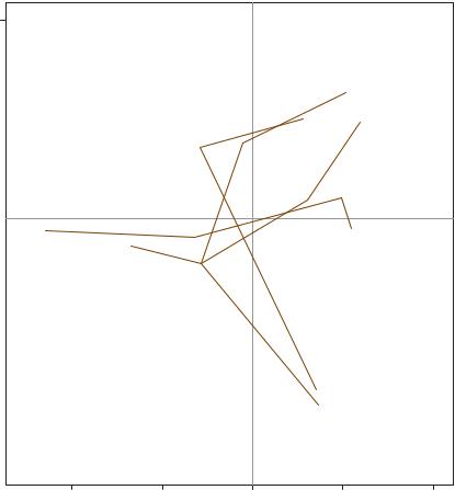
Exhibit 11.7:

Fuzzy categories of the four environmental variables, positioned at their respective weighted averages of the samples. The sample ordination is given in Exhibit 11.3, and linear relationships of species and variables in Exhibit 11.5

MULTIVARIATE ANALYSIS OF ECOLOGICAL DATA

0.4

					t1
	0.2			Lat4	Lon4
				Lat3
				t2
				Lon3	d2
Dimension2	0.0		d4	d3	d1
				t3 Lon2
				Lon1
				Lat2
	–0.2

Lat1

–0.4		t4

–0.4

–0.2

0.0

0.2

0.4

Dimension 1

categories differs depending on the temperature category. Another example is the pair of variables latitude and longitude: in both Exhibits 11.5 and 11.7, it is not possible to determine if the effect of longitude is contingent on latitude. In regular statistical modelling involving continuous variables, an interaction is coded by the product of the two variables and this product is included in the model as well as the linear terms. But for our purpose, showing gradient vectors in an MDS ordination for the linear terms of latitude and longitude and for their product is very difficult to interpret (the same problem occurs if one codes polynomial terms of latitude and longitude, which is often recommended to account for a nonlinear spatial component – the biplot representation of powers and cross-products of latitude and longitude coordinates is hard to interpret).

146

MULTIDIMENSIONAL SCALING BIPLOTS

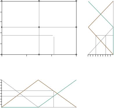
Fuzzy coding offers a better alternative, shown in Exhibit 11.8. The fuzzy coding of latitude and longitude (or any other pair of variables whose interaction needs to be explored) is computed, giving two sets of three numbers as shown, and then all pairs of these numbers give nine fuzzy categories coding the eight compass points and a central category. For two continuous variables such as depth and temperature, the eight outer categories would code, for example, depth and temperature high (“north-eastern” category), temperature near the centre, depth high (“eastern” category, if depth is considered on the horizontal axis of the scheme in Exhibit 11.8), temperature low and depth high (“south-eastern” category), and so on. Finally, for the spatial variables, Exhibit 11.9 shows the positions of the nine categories. The points are connected by lines which would form a square grid if no interaction were present. There is a clear interaction, with the eastern regions having less difference than the western regions. This is a richer result than showing latitude and longitude by two simple vectors, and reflects the more complex nature of the relationship of fish abundances to the geography.

75			Category 3	75
71.8		×	Category 2	71.8 72.5	Latitude
			1
70			Category	70
		41	1	0
20	30	40	50

1	Category 1	Category 2		Category 3		0
						0.72		0	0.6	0.4
					0.28
						0		0		0
				=		0	0.432		0.288
0					0		0.168		0.112
	20	35	41.0	50
		Longitude

Exhibit 11.8:

Coding the latitude– longitude interaction into fuzzy categories: for

example, each is coded into three fuzzy categories and then all pairwise products of the categories are computed to give nine categories coding the interaction. For example, the point with latitude 71.8ºN and longitude

41ºE has fuzzy coding [0.28 0.72 0] and

[0 0.6 0.4] respectively. The first set is reversed

to give values from north to south, and all combinations of the fuzzy values give nine categories coding the eight compass points and a central location

147

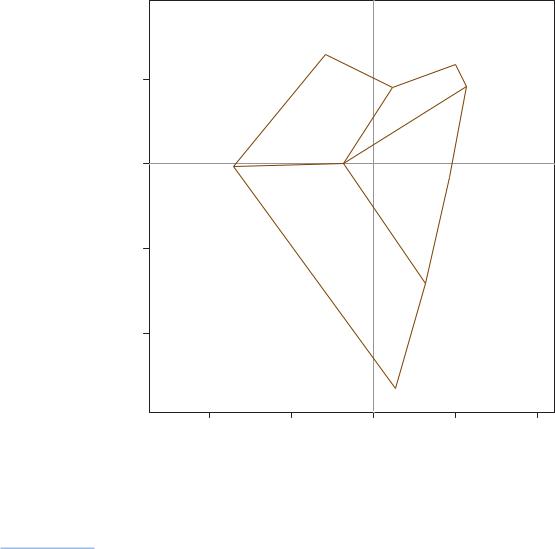
Exhibit 11.9:

The positions of the nine fuzzy categories coding the interaction between latitude and longitude. Labels are the eight compass points, and C for central position

0.2

Dimension 2 –0.2 0.0

–0.4

MULTIVARIATE ANALYSIS OF ECOLOGICAL DATA

NW

NE

N

E

W

C

SE

S

SW

–0.4

–0.2

0.0

0.2

0.4

Dimension 1

SUMMARY: Multidimensional scaling biplots

1.Multidimensional scaling (MDS) makes an ordination map of a matrix of proximities within a set of samples, based on variables observed in each sample, for example species abundances, environmental or geographical variables, and so on.

2.Once this ordination map is achieved, the variables on which it was originally based can be related to the dimensions of the map using the regression biplot approach, whereby regression models are fitted to each variable as a response and the ordination dimensions as predictors.

3.When the spatial coordinates of the samples are known, it is relevant to relate the ordination map to the spatial map. This can be done either by comparing inter-sample spatial distance with inter-sample distance in the ordination map, or by performing Procrustes analysis on the two configurations.

148

MULTIDIMENSIONAL SCALING BIPLOTS

4.The nonlinear contours of a concomitant continuous variable observed on all the samples can also be visualized, one at a time, and compared to the straightline contours implied by the regression biplot.

5.Fuzzy coding is useful for visualizing these nonlinear contours in a simple way that allows several variables to be visualized simultaneously.

6.Fuzzy coding can also be used to code interactions between continuous variables, such as latitude and longitude, and thus enrich the interpretation of the MDS result.

149