

диафрагмированные волноводные фильтры / 2557f7e0-586a-4a6d-9fda-53c945c07f90
.pdfE-plane resonators for compact inline waveguide filters
UJankovic*, N Mohottige†, D Budimir*
*University of Westminster, London, UK, d.budimir@westminster.ac.uk, † Cobham Wireless, Chesham, UK
Keywords: waveguide filters, Q factor.
Abstract
Waveguide resonators incorporating E-plane metal inserts with fins have already been demonstrated in building extracted pole sections (EPSs) for very compact and easily fabricated microwave filters. Flexibility of transmission poles (TPs) and zeros (TZs) locations for different resonant and non-resonant modes is further shown and the electromagnetic nature of these modes as well as natural frequencies of EPS sections are explained and numerically estimated. Detailed comparison with conventional waveguide resonators, overmoded cavities, state of the art waveguide resonator solutions and substrate intergerated waveguide resonators is performed at 10 GHz.
1 Introduction
Even though waveguide technology had its initial most significant development in the first half of the 20th century, it is still unparalleled when it comes to applications requiring low loss, high power and perfect EM isolation. Moreover, during time, demands for compactness, complex filter networks with very low insertion loss and high roll-off have been pushed ever closer to the obtainable physical limits. Also, new system requirements such as millimetre wave links for 5G mobile networks as well as new fabrication technologies and implementations like substrate integrated waveguide (SIW) one are always bringing freshness to the area.
In [1] Konishi and Uenakada proposed use of metal E-plane inserts for realisation of directly coupled waveguide filters [2]. E-plane waveguide technology is likewise very suitable for implementation of ridged waveguide resonators [3] and quasi-lowpass corrugated-waveguide filters [4]. In [5], the size of the conventional E-plane resonator was reduced and transmission zero introduced through the addition of metal S- shaped lines on dielectric slab. Finally, in [6] extracted pole sections using fins have been introduced. Further miniaturization was achieved by use of several fins [7], and multiplexers based on this filter structure have been designed [8]. In this paper, compact E-plain resonators with fins are explored in more details regarding their fundamental characteristics, resonant frequencies and quality factors, as well as for their power handling capability as one of the chief characteristics of resilience of these microwave components in real life applications.
2 Resonator structure
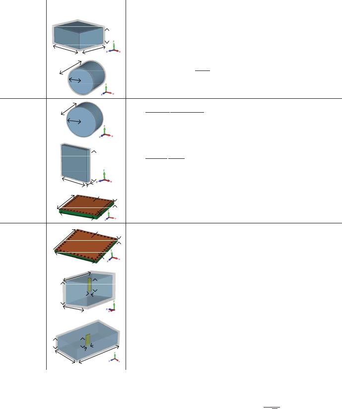
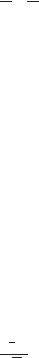
3D model of an E-plane inline resonator with fin coupled on both sides to form an EPS section is shown in Fig 1a, whereas its equivalent scheme is depicted in Fig 1b. That is, the central fin can be represented by a parallel connected serious LC circuit, the waveguide straight sections around it by equivalent transmission line sections having the same characteristic impedance as the waveguide wave impedance, and the enclosing septa as immitance invertors.
Ă>ĨŝŶ
tĨŝŶ
ď
Ă
Ő |
D^͕ϭ |
> |
|
Z> |
|
ZƐ |
|
Dϭ͕> |
|||
|
|||||
͕ Đ |
|
͕ Đ |
|
||
|
|
|
ď
Figure 1: a) 3D model of proposed E-plane inline resonator and b) its equivalent circuit
The dominant mode is based on TE101 mode, which can be observed by half sine field oscillations in x and z directions. In horizontal plane, electric field diminishes on all the side walls, while in the central part, where it is the strongest, it surround the fin and is much tighter localized than it is for the resonator without a fin. Adding the fin, which effectively meanders the EM field inside the cavity, can be represented as a continuous transformation of the top waveguide wall.
3 Resonances
First of all, the fin length will be extracted from the TZ position. Transmission zeros are inherent property of a transmission function of a network between two of its ports. They tell at which (complex) frequencies the ports are decoupled. For that reason, it does not matter how are these
1
two ports closed – if we inspect the transfer function relation for that pair of ports through different parameters (Z,Y,S) it will have exactly the same transfer function numerator zeros if we do not take into the account possible cancellation effect. In other words, there is a cut in the signal path. This directly implies that we can extract EPS section zeros by removing invertors, that is, just keeping the fin inside a waveguide. In practice, this can be affected by mutual coupling of the fin with other elements, in this case septa and other fins, which becomes more significant as the structure’s size reduces.
For ideally thin fin, its length can be approximately calculated by the expression:
Lfin=0.287ÂȜ – 0.065Âa |
(1) |
So, the fin length is very slightly larger than the quarter wavelength. Here, Ȝ=c/f is a free space wavelength rather than the guided one. This can be explained by the fact that the fin lays in a cross section plane and not along the waveguide. And by image theory applied on waveguide walls, the fin transforms into 2D array of half-wavelength dipoles in open space. Hence in theory, at the cut-of frequency, the fin length is roughly equal to the waveguide height.
Metal insert is supposed to be thin (< 2% a), but thicker than the skin depth so that perturbation method can be applied. Then, it can be taken that insert thickness does not influence the transmission zero frequency.
Including the fin width Wfin, TZ frequency can be roughly calculated by
f z |
= |
0.287 c |
|
+ f |
c |
Wfin |
, |
(2) |
|
Lfin + 0.065 |
a |
a |
|||||||
|
|
|
|
||||||
|
|
|
|
|
|
where fc is the waveguide cut-off frequency. Estimating Wfin, which enlarging reduces the coupling and narrows the bandwidth, Lfin can easily be found from the TZ frequency fz calculated in the ideal model to satisfy the specification.
In frequency band where higher order modes start to appear, first there is a visible shift in fin length, and at about 3Ȝ/4, secondary radiation from the fin is mostly transferred to higher modes with first index odd (odd number of half-sine oscillations along the wider cross section rectangle edge due to the location of the fin in the centre which fixes field
maximum in that position), i.e. TE11, TM11, TE30,… in the order they appear. Accordingly, TZ effect in the dominant
mode diminishes. Since for historical reasons the wider rectangle side is a bit more than double length of the shorter one, these spurious modes are further shifted to higher frequencies, i.e. more than twice the cut-off frequency of the dominant mode. E.g. for X-band WR-90 , cut-off frequencies of TE11 and TM11 modes are 16.16 GHz.
Pole resonant frequency in an unloaded resonator can be calculated starting with the ubiquitous expression for the TE101 mode in the rectangular waveguide cavity, modifying it through division with a nonlinear function larger or equal
than one, which depends on Lfin and has relatively modest steepness for small values of Lfin, but it increases afterwards. Nevertheless, of interest are only those larger values of Lfin for which this function can be linearized. Except for Wfin that can vary in a large band, small changes with all parameters fixed apart from one make roughly linear changes, meaning that partial derivatives of frequency are nearly constant in the ranges of interest.
Therefore, using least square method to approximate overdeterminate system of linear equations, for thin fin the transmission pole frequency in X band can be estimated by:
fp [GHz] = |
(3) |
26.5 - 0.68ÂL[mm] - (2.13-0.073ÂL[mm])ÂLfin[mm]
Since Lfin is already known from satisfying TZ location, it is not difficult to calculate L from the known TP frequency.
Transmission poles from the transmission network are isolated by eigenmode solver, as they are the natural frequencies when the network ports are short circuited. There may be a confusion arising by the asymmetric properties of TPs and TZs. If we take as an example a reflexion parameter, there is indeed symmetry between the denominator and the numerator, since two different reflection parameters are just inverse one to another. But this is just an exception which does not violate the more universal property of not having symmetry between the denominator and the numerator. It is important to stress that the mathematical function through which we can observe the natural frequencies (complex in general case) is a transfer function, which in strictly a response function over a source function in the Laplace domain. This signifies that although in both denominator and numerator of a transfer function we have polynomials, there is no symmetry in the general case between them – the fundamental characteristic of a circuit lays in the zeros of the denominator, not the numerator.
3.1 Higher order modes
In [6] are as well used higher order modes, put together to form dual-mode resonator. Actually, these are not degenerate modes, but modes of very different nature, though are of similar resonant frequencies. First one is modification of TE101 mode, just as the dominant mode (for both modes it can be checked that varying a and d alters the resonant frequency, whereas changing b has only minuscular indirect effect over the fin), however, with a different mode in the volume around the fin. This can be view by comparison of the field distributions at the foot of the fin for these two modes, fig. 2. While one has electric field lines going into the corner like rays of cylindrical waves (a) to satisfy no tangent electric field component boundary condition, the other has electric field lines forming arcs centred on the fin slightly below the waveguide top wall (b). The second mode in the transmission pole pair is almost unaltered TE102 mode due to the fact that the fin is positioned where the field has its minimum. This also means that changing fin length, while having large effect
2

on the neighbouring transmission pole and transmission zero, |
As the rectangular waveguide is used the standard X-band |
|||||||||||||||||||||||||||||||||||||||||||||||||||||||||||||||||||||||||||||||||||
has negligible effect on the transmission pole resulting from |
WR-90 having cross section dimensions |
|
|
|
|
|
|
|
|
|
|
mm and |
||||||||||||||||||||||||||||||||||||||||||||||||||||||||||||||||||||||||
this cavity resonance. These properties allow various different |
|
|
|
|
|
|
|
|
|
|
||||||||||||||||||||||||||||||||||||||||||||||||||||||||||||||||||||||||||
|
|
|
|
|
|
|
|
|
|
|
mm to accommodate the |
dominant TE |
|
|
||||||||||||||||||||||||||||||||||||||||||||||||||||||||||||||||||||||
responses such as transmission pole-zero-pole sequence. |
|
|
|
|
|
|
|
|
|
|
|
|
|
|||||||||||||||||||||||||||||||||||||||||||||||||||||||||||||||||||||||
|
|
|
|
|
|
|
|
|
|
|
|
ʹʹǤͺ101 mode |
||||||||||||||||||||||||||||||||||||||||||||||||||||||||||||||||||||||||
|
|
|
|
|
|
|
|
|
|
|
|
|
|
|
|
|
|
|
|
|
|
|
|
|
|
|
|
|
|
|
|
|
|
|
|
|
resonant cavity, being guided by its inline applications such |
|||||||||||||||||||||||||||||||||||||||||||||||
|
|
|
|
|
|
|
|
|
|
|
|
|
|
|
|
|
|
|
|
|
|
|
|
|
|
|
|
|
|
|
|
|
|
|
|
|
Ǥ |
|
|
|
|
|
|
|
|
|
|
|
|
|
|
|
|
|
|
|
|
|
|
|
|
|
|
|
|
|
|
|
|
|
|
|
|
|||||||||||
|
|
|
|
|
|
|
|
|
|
|
|
|
|
|
|
|
|
|
|
|
|
|
|
|
|
|
|
|
|
|
|
|
|
|
|
|
as in directly coupled waveguide |
|
filters |
[1], |
|
[2]. |
|
From |
||||||||||||||||||||||||||||||||||||||||
|
|
|
|
|
|
|
|
|
|
|
|
|
|
|
|
|
|
|
|
|
|
|
|
|
|
|
|
|
|
|
|
|
|
|
|
|
|
|
|
|
|
|
|
|
|
|
|
|
|
|
|
|
|
|
is |
calculated |
the |
|
|
rectangular |
||||||||||||||||||||||||
|
|
|
|
|
|
|
|
|
|
|
|
|
|
|
|
|
|
|
|
|
|
|
|
|
|
|
|
|
|
|
|
|
|
|
|
|
waveguide cavity |
length |
|
|
|
|
|
|
|
|
|
|
|
|
|
|
|
|
|
|
|
|
|
mm. |
|
|
||||||||||||||||||||||
|
|
|
|
|
|
|
|
|
|
|
|
|
|
|
|
|
|
|
|
|
|
|
|
|
|
|
|
|
|
|
|
|
|
|
|
|
|
|
|
|
|
|
|
|
|
|
|
|
|
ͻǤͺ |
|
|
|
|
|
|||||||||||||||||||||||||||||
|
|
|
|
|
|
|
|
|
|
|
|
|
|
|
|
|
|
|
|
|
|
|
|
|
|
|
|
|
|
|
|
|
|
|
|
|
|
|
|
|
|
|
|
|
|
|
|
|
|
|
|
|
|
|
|
|
|
|
|
|
|
|
|
|
|
|
|
|
||||||||||||||||
|
|
|
|
|
|
|
|
|
|
|
|
|
|
|
|
|
|
|
|
|
|
|
|
|
|
|
|
|
|
|
|
|
|
|
|
|
|
|
|
|
|
|
|
|
|
|
|
|
|
|
|
|
|
|
|
|
|
|
|
|
|
|
|
|
|
|||||||||||||||||||
|
|
|
|
|
|
|
|
|
|
|
|
|
|
|
|
|
|
|
|
|
|
|
|
|
|
|
|
|
|
|
|
|
|
|
|
|
|
|
|
|
|
|
|
|
|
|
|
|
|
|
|
|
|
|
|
|
|
|
|
|
|
|
|
|
|
|
|
|
|
|
|
|
|
|
|
|
|
|
|
|
|
|
|
|
|
|
|
|
|
|
|
|
|
|
|
|
|
|
|
|
|
|
|
|
|
|
|
|
|
|
|
|
|
|
|
|
|
|
|
|
|
Use of degenerate TM120 and TM210 modes was proposed in |
|||||||||||||||||||||||||||||||||||||||||||||||
|
|
|
|
|
|
|
|
|
|
|
|
|
|
|
|
|
|
|
|
|
|
|
|
|
|
|
|
|
|
|
|
|
|
|
|
|
[11] for the sake of having design flexibilities in terms of the |
|||||||||||||||||||||||||||||||||||||||||||||||
|
|
|
|
|
|
|
|
|
|
|
|
|
|
|
|
|
|
|
|
|
|
|
|
|
|
|
|
|
|
|
|
|
|
|
|
|
number and position of transmission zeros, response |
|||||||||||||||||||||||||||||||||||||||||||||||
Figure 2: Electric field lines in the central waveguide E-plane |
bandwidth as well as of the cavity length. The latter is |
|||||||||||||||||||||||||||||||||||||||||||||||||||||||||||||||||||||||||||||||||||
because |
of |
having |
|
the |
last |
mode |
|
|
index |
referring |
to the |
|||||||||||||||||||||||||||||||||||||||||||||||||||||||||||||||||||||||||
cross section at the fin bottom for a) dominant and b) second |
longitudinal direction zero. The rectangular waveguide cavity |
|||||||||||||||||||||||||||||||||||||||||||||||||||||||||||||||||||||||||||||||||||
TE101 modes. |
|
|
|
|
|
|
|
|
|
|
|
|
|
|
|
|
|
|
|
|
|
|
|
|
|
|
|
|
|
|
|
|||||||||||||||||||||||||||||||||||||||||||||||||||||
|
|
|
|
|
|
|
|
|
|
|
|
|
|
|
|
|
|
|
|
|
|
|
|
|
|
|
|
|
|
|
accommodating TM120 and TM210 modes is set to have |
|||||||||||||||||||||||||||||||||||||||||||||||||||||
|
|
|
|
|
|
|
|
|
|
|
|
|
|
|
|
|
|
|
|
|
|
|
|
|
|
|
|
|
|
|
|
|
|
|
|
|
||||||||||||||||||||||||||||||||||||||||||||||||
3 |
|
Q factor |
|
|
|
|
|
|
|
|
|
|
|
|
|
|
|
|
|
|
|
|
|
|
|
|
|
|
|
|
|
|
|
dimensions exactly like in [11] where resonant frequency is |
||||||||||||||||||||||||||||||||||||||||||||||||||
|
|
|
|
|
|
|
|
|
|
|
|
|
|
|
|
|
|
|
|
|
|
|
|
|
|
|
|
|
|
|
|
already 10 GHz (since the resonant frequency is independent |
||||||||||||||||||||||||||||||||||||||||||||||||||||
Comparison of (unloaded) Q factors for different cavity |
of |
|
|
|
d, |
for |
|
equal |
|
sides a |
and |
|
|
b, |
|
|
|
|
|
ξ |
|
), |
hence |
|||||||||||||||||||||||||||||||||||||||||||||||||||||||||||||
resonators at f = 10 GHz is given in Table 1. |
|
|
|
|
|
|
|
|
|
|
|
|
|
|
|
|
|
|
|
|
|
|
|
|
|
|
|
and |
|
|
|
|
|
|
|
|
|
|
|
|
|
|
|
When calculated |
||||||||||||||||||||||||||||||||||||||||
Here, |
|
universally, |
|
|
|
|
|
|
|
|
|
|
|
x |
|
|
|
|
|
|
|
|
|
and |
|
|
|
|
|
|
|
|
|
|
|
|
|
|
|
|
|
|
|
|
|
|
|
|
|
|
|
|
|
|
|
|
. |
|
|
|
||||||||||||||||||||||||
|
|
|
|
|
|
|
|
|
|
|
|
|
|
|
|
|
|
|
|
|
|
|
|
|
|
|
|
|
|
|
|
is scaled by the factor |
|
|
|
|
|
|
, which corresponds |
|||||||||||||||||||||||||||||||||||||||||||||
|
|
|
|
|
|
|
|
|
|
|
|
|
|
|
|
|
|
|
|
|
|
|
|
|
|
|
|
|
|
|
|
|
|
|
͵͵Ǥ ʹ |
|
|
|
|
|
Ǥ |
|
|
|
|
|
|
|
|
|
|
|
|
|||||||||||||||||||||||||||||||
|
|
|
|
|
|
|
|
|
|
|
|
|
|
|
|
|
|
|
|
|
|
|
|
|
|
|
|
|
|
|
|
|
|
|
|
|
|
|
|
|
|
|
|
|
|
|
|
|
|
|
|
|
|
|
|
|
|
|
|
|
|
|
|
|
|
|
|
|
|
|
|
|
|
|
|
|
|
|
||||||
|
|
|
|
|
|
|
|
|
|
|
|
|
|
|
|
vacuum |
|
permittivity |
and |
vacuum |
|
|
|
|
|
|
|
|
|
|
|
|
|
|
|
|
|
|
|
|
|
|
|
|
|
|
|
|
|
|
|
|
|
|
|
|
|
|
|
|
|
|
|
|
|
|
|
|
||||||||||||||||
|
|
|
|
x |
|
|
|
|
|
|
|
|
are |
|
|
|
ɂ |
|
|
ͺǤͺ |
|
|
|
|
|
|
|
|
|
|
|
|
|
|
|
|
|
|
|
|
|
|
|
|
|
|
|
|
|
|
|
|
|
|
|
|
|
|
|
|
|
|
|
|
|
|
|
|
the resulting |
|||||||||||||||
|
|
|
|
|
|
|
|
|
|
|
|
|
|
|
|
|
|
|
|
|
|
|
|
|
|
|
|
|
|
|
|
|
|
|
|
|
|
|
|
|
|
|
|
|
|
|
|
|
|
|
|
|
|
|
|
|
|
|
|
|||||||||||||||||||||||||
|
|
|
|
|
|
|
|
|
|
|
|
|
|
|
|
|
|
|
|
|
|
|
|
|
|
|
|
|
|
|
|
|
|
|
|
to using silver plating instead of pure aluminium, |
||||||||||||||||||||||||||||||||||||||||||||||||
Ɋ Ɏ |
|
|
|
|
|
|
|
|
|
|
|
|
|
|
|
|
|
|
|
|
͵ Ǥ ͵ π |
Qu |
|
is 5505.1, which is close to the value 5550 given in the |
||||||||||||||||||||||||||||||||||||||||||||||||||||||||||||
|
|
|
|
|
|
|
|
|
|
|
|
|
|
|
|
|||||||||||||||||||||||||||||||||||||||||||||||||||||||||||||||||||||
permeability constants respectively, |
|
|
paper. |
|
|
|
|
|
|
|
|
|
|
|
|
|
|
|
|
|
|
|
|
|
|
|
|
|
|
|
|
|
|
|
|
|
|
|
|
|
|
|
||||||||||||||||||||||||||||||||||||||||||
|
|
|
|
|
|
|
|
|
|
|
|
|
|
|
|
|
|
|
|
|
|
|
|
|
|
|
|
|
|
|
|
|
|
|
|
|
|
|
|
|
|
|
|
|
|
|
|
|
|
|
|
|
|
|
|
|
|
|
|
|
|
|
|
|
||||||||||||||||||||
is |
|
impedance of |
|
|
free |
|
space, |
|
|
|
|
|
|
|
|
|
is |
angular |
|
|
|
|
|
|
|
|
|
|
|
|
|
|
|
|
|
|
|
|
|
|
|
|
|
|||||||||||||||||||||||||||||||||||||||||
|
|
|
|
|
|
|
|
|
|
|
|
|
|
As the circular waveguide is used X-band C104 waveguide |
||||||||||||||||||||||||||||||||||||||||||||||||||||||||||||||||||||||
|
|
|
|
|
|
|
|
|
|
|
|
|
|
|
|
|
|
|
|
|
|
|
|
|
|
|
|
|
|
|
|
|
||||||||||||||||||||||||||||||||||||||||||||||||||||
wavenumber and |
|
|
|
|
|
|
|
|
|
|
|
|
is surface resistance. |
|
|
|
|
|
|
|
|
|
|
|
|
|
|
|
|
|
|
|
|
|
|
|
|
|
|
|
|
|
|
|
|
|
|
|
|
|
|
|
|
|
|
|
|
|
|
|
|
|
||||||||||||||||||||||
|
|
|
|
|
|
|
|
|
|
|
|
|
|
|
|
|
|
|
|
|
|
|
|
|
|
|
|
|
|
|
|
|
|
|
|
|
|
|
|
|
|
|
|
|
|
|
|
|
|
|
|
|
|
|
|
|
|
|
|
|
||||||||||||||||||||||||
|
|
|
|
|
|
|
|
|
|
|
ɘ ɂ Ɋ |
|
|
|
|
|
having inner radius of |
|
|
|
|
|
|
|
|
|
|
|
mm to accommodate the |
|||||||||||||||||||||||||||||||||||||||||||||||||||||||
|
|
|
|
|
|
|
|
|
|
|
|
|
|
|
|
|
|
|
|
|
|
|
|
|
|
|
dominant TE111 mode resonant cavity, being guided by its |
|||||||||||||||||||||||||||||||||||||||||||||||||||||||||
Regarding material properties, it is assumed that metal |
|
|
|
|
|
|
|
|
|
|
|
|
|
|
|
|
|
|
|
Ǥ ʹʹ |
|
|
|
|
|
|
|
|
|
|
|
|
|
|
|
|
|
|||||||||||||||||||||||||||||||||||||||||||||||
|
|
|
|
|
|
|
|
|
|
|
|
|
|
|
|
|
|
|
|
|
|
|
|
|
|
|
|
|
|
|
||||||||||||||||||||||||||||||||||||||||||||||||||||||
waveguide |
x |
housings |
|
|
|
are |
|
|
made |
|
of |
|
|
|
aluminium, |
inline |
|
applications. From |
|
|
|
|
|
|
|
|
|
|
|
|
|
, |
||||||||||||||||||||||||||||||||||||||||||||||||||||
|
|
|
|
|
|
|
|
, |
|
|
|
|
|
|
|
|
|
m , and metallic inserts of |
|
|
|
|
|
|
|
|
|
|
|
|
, is |
calculated |
the |
circular |
|
waveguide |
cavity |
|||||||||||||||||||||||||||||||||||||||||||||||
|
|
|
|
|
|
|
|
|
|
|
|
|
|
|
|
|
|
|
|
|
|
|
|
|
|
|
|
|
|
|
|
|
|
|
|
|
|
|
|
|
|
|
|
|
|
|
|
|
|
|
|
|
|
|
|
|
|
|
|
|
|
|
|
|
|
|
|
|
||||||||||||||||
|
|
|
|
|
|
|
|
|
|
|
|
|
|
|
|
|
|
|
|
|
|
|
|
|
|
|
|
|
|
|
|
|
|
length, |
|
|
|
|
|
|
|
|
|
|
|
|
|
|
|
|
|
|
|
|
|
|
|
|
mm.. |
|
In |
|
|
addition, |
||||||||||||||||||||
|
|
|
|
|
|
|
|
|
|
|
|
|
|
|
|
|
|
|
|
|
|
|
|
|
|
|
|
|
|
|
|
|
|
|
|
|
|
|
|
|
|
|
|
|
|
|
|
|
|
|
|
|
|
|
|
|
|
|
|
|
|
|
|
|
|
|
|
|
|
|
|
|
|
|
|
|
|
|
|
|||||
annealed |
|
copper, |
|
|
͵͵Ǥx |
|
π |
|
|
|
|
|
|
|
|
|
|
|
|
|
|
|
|
Ǥͺ |
|
|
|
|
|
|
|
|
|
|
|
|
|
|
|
|
|
|
|
|
|
|
|
|
|
|
|
|
|
|
|
|
|
|
|
|
||||||||||||||||||||||||
|
|
|
|
|
|
|
|
|
|
|
|
|
|
|
|
|
|
|
|
|
|
|
|
|
|
|
|
|
|
|
|
|
|
|
|
|
|
|
|
|
|
|
|
|
|
|
|
|
|
|
|
|
|
|
||||||||||||||||||||||||||||||
|
|
|
|
|
|
|
|
|
|
|
|
|
|
|
|
|
|
|
|
|
|
|
|
|
|
|
|
|
|
|
|
|
|
|
|
|
|
|
|
|
|
|
|
|
|
|
|
|
|
|
|
|
|
|||||||||||||||||||||||||||||||
|
|
|
|
|
. |
|
In |
|
SIW |
design, |
|
|
|
|
|
|
|
|
|
|
|
|
|
|
|
|
|
|
|
|
|
|
|
|
|
|
|
|
|
|
|
|
|
|
|
|
||||||||||||||||||||||||||||||||||||||
ɐ |
|
͵Ǥ |
|
|
|
|
|
|
|
|
|
|
|
|
|
|
|
|
|
|
͵ Ǥ |
|
|
|
|
|
|
|
|
|
|
|
|
|
|
|||||||||||||||||||||||||||||||||||||||||||||||||
|
|
|
|
|
|
|
|
|
|
|
|
|
low loss Rogers RT/duroid 5880 high |
|
|
|
|
|
|
|
|
|
|
|
|
|
|
|
|
|
|
|
|
|
|
|
|
|
|
|
|
|
|
|
|
|||||||||||||||||||||||||||||||||||||||
hsub = 1.575 mm thick |
|
|
|
|
|
|
|
|
|
|
|
|
|
|
|
|
|
|
|
|
|
|
|
|
|
|
|
|
|
|
|
|
|
|
|
|
|
|
|
|
|
|
|
|
|
|
|
|
||||||||||||||||||||||||||||||||||||
|
|
|
|
|
|
|
|
|
|
|
ɐ |
Ǥͺ |
|
|
|
|
|
|
|
|
|
|
|
|
|
|
|
|
|
|
|
|
|
|
|
|
|
|
|
|
|
|
|
|
|
|
|
|
|
|
|
|
|
|
|
|
|
|
|
|
|
|||||||||||||||||||||||
frequency |
|
laminate |
|
is |
|
|
used |
|
having relative |
|
permittivity |
|
TE |
|
|
|
|
|
|
|
|
|
|
|
|
|
|
|
|
|
. |
|
|
|
|
|
|
|
|
|
|
|
|
|
|
|
|
|
|
|
|
|
|
|
|
|
|
|||||||||||||||||||||||||||
|
|
|
|
|
|
Ⱦ |
|
|
|
|
|
|
|
|
|
|
|
|
|
|
|
|
|
|
|
|
|
|
|
|
|
|
|
|
||||||||||||||||||||||||||||||||||||||||||||||||||
|
|
|
|
and |
|
|
|
|
|
|
|
|
|
|
|
|
|
|
|
|
dielectric |
|
characteristics. |
|
|
|
|
|
|
|
|
|
|
|
|
|
|
|
|
|
|
|
|
|
|
|
|
|
|
|
|
|
|
|||||||||||||||||||||||||||||||
Copper |
cladding |
|
|
has |
|
|
|
|
|
|
|
|
|
|
|
|
|
|
thickness with |
In |
|
contrast, |
the |
overmoded |
cavity |
|
|
accommodating |
TE011 |
|||||||||||||||||||||||||||||||||||||||||||||||||||||||
ɂ ʹǤʹ |
|
|
|
|
|
Ɂ Ǥ ͻ |
|
|
|
|
|
|
|
|
|
|
|
|
|
|
|
mode is scaled to have proportions like the average cavity in |
||||||||||||||||||||||||||||||||||||||||||||||||||||||||||||||
|
|
|
|
|
|
|
|
|
|
|
|
|
|
|
|
|
|
roughness on the dielectric side |
||||||||||||||||||||||||||||||||||||||||||||||||||||||||||||||||||
|
|
|
|
|
|
|
RMS surfaceݐ Ǥ Ɋ |
|
|
|
|
|
|
|
|
|
|
[10], |
|
|
|
|
|
|
|
|
|
. Having |
|
|
|
|
|
|
|
|
|
|
|
|
|
, |
|
|
|
|
|
|
|
|
|
|||||||||||||||||||||||||||||||||
for electrodeposited copper to result in effective conductivity |
|
|
|
|
|
|
|
|
|
|
|
|
|
|
|
|
|
|
|
|
|
|
|
|
|
|
|
|
|
|||||||||||||||||||||||||||||||||||||||||||||||||||||||
Ǥͺ Ɋ |
|
|
|
|
|
|
|
|
|
|
|
|
|
|
|
|
|
|
|
|
|
|
|
|
|
|
|
|
|
|
|
|
|
|
|
|
|
|
|
|
|
|
|
|
|
|
|
|
|
|
|
|
|
|
|
|
|
|
|
|
|
|
|
|
|
|
|
|
|
|
|
|
|
|
|
|||||||||
of |
|
ǡ |
|
|
|
|
|
|
|
x |
|
|
|
|
|
|
. |
|
|
|
|
|
|
|
|
|
|
|
|
|
|
|
|
|
|
and |
|
|
|
|
|
Ǥ ͺmm is calculated. ͵Ǥͺ͵ʹ |
|
|
ʹʹǤ |
|||||||||||||||||||||||||||||||||||||||
|
ɐ |
ʹǤ |
|
|
|
|
|
|
|
|
|
|
|
|
|
|
|
|
|
|
|
|
|
|
|
|
|
|
|
|
|
|
|
|
|
|
|
|
|
|
|
|
|
|
|
|
|
|
|
|
|
|
|
|
|
|
|
|
|
|
|
|
|
|
|
|
|
|
|
|
|
|
|
|
|
|
||||||||
3
Cavity type |
|
Model |
|
|
|
|
Calculation method |
|
|
|
|
|
|
|
|
|
|
|
|
Q |
|
Volume |
|
Τ |
||||||||||||||||||||||||||||||||
Rectangular |
|
|
|
|
|
|
|
|
|
|
|
|
|
|
|
|
|
|
|
|
|
|
|
|
|
|
|
|
|
|
|
|
|
|
|
|
|
|
|
|
|
|
|
|
|
|
|
value |
|
V[mm3] |
|
|||||
(mode) |
|
|
|
|
|
|
|
|
|
|
|
|
|
|
|
|
|
|
|
|
|
|
|
|
|
|
|
|
|
|
|
|
|
|
|
|
|
|
|
|
|
|
|
|
|
|
|
|
|
|
|
mm |
|
|||
cavity |
|
|
|
|
|
|
|
|
|
|
|
|
|
|
|
|
|
|
|
|
|
|
|
|
|
|
|
|
|
|
|
|
|
|
|
|
|
|
|
|
|
|
|
|
|
|
||||||||||
waveguide |
|
|
|
|
|
|
|
|
|
|
|
|
|
|
|
|
|
|
|
|
|
|
|
|
|
|
|
|
|
|
|
|
|
|
|
|
|
|
|
|
|
|
|
|
|
Ǥͻ |
|
Ǥ |
|
|
Ǥ͵ʹ |
|
||||
|
|
|
|
|
|
|
|
|
|
|
|
|
|
|
|
|
|
|
|
|
|
|
|
|
|
|
|
|
|
|
|
|||||||||||||||||||||||||
(TE101 |
mode) |
|
|
|
|
|
|
|
|
|
|
|
|
|
|
|
|
|
|
|
|
|
|
|
|
|
|
|
|
|
||||||||||||||||||||||||||
|
|
|
|
|
|
|
|
|
|
|
|
|
|
|
|
|
|
|
|
|
|
|
|
|
|
|
|
|||||||||||||||||||||||||||||
[9], Sec. 6.3 |
|
|
|
|
|
|
|
|
|
|
|
|
|
|
|
|
|
|
|
|
ή ή |
|
|
|
|
|
|
|
|
|
|
|
|
|
|
|
|
|
|
|
|
|
|
|||||||||||||
Circular |
|
|
|
|
|
|
|
|
|
|
|
|
|
|
|
|
|
|
|
|
|
|
|
|
|
|
|
|
|
|
|
|
|
|
|
|
|
|
|
|
|
|
|
|
|
|
|
|
|
|
||||||
waveguide |
|
|
|
|
|
|
|
|
|
|
|
|
|
|
|
|
|
|
|
|
|
|
|
|
|
|
|
|
|
|
|
|
|
|
|
|
|
|
|
|
|
|
|
|
|
|
|
|
|
|
|
|
|
|||
cavity |
|
|
|
|
|
|
|
|
|
|
|
|
|
|
|
|
|
|
|
|
|
|
|
|
|
|
|
|
|
|
|
|
|
|
|
|
|
|
|
|
|
|
|
|
|
|
|
|
|
|
|
|
||||
|
|
|
|
|
|
|
|
|
|
|
|
|
|
|
|
|
|
|
|
|
|
|
|
|
|
|
|
|
|
|
|
|
|
|
|
|
|
|
|
ͺͺͻ |
|
ͻ |
|
|
Ǥͻʹ |
|
||||||||||
(TE111 mode) |
|
|
|
|
|
|
|
|
|
|
|
|
|
|
|
|
|
|
|
|
|
|
|
|
|
|
|
|
|
|
|
|
|
|
|
|
|
|
|
|||||||||||||||||
|
|
|
|
|
|
|
|
|
|
|
|
|
|
|
|
|
|
|
|
|
|
|
|
|
|
|
|
|
|
|
|
|
|
|
|
|
|
|
|
|
|
|||||||||||||||
|
|
|
|
|
|
|
|
|
|
|
|
|
|
|
|
|
|
|
|
|
|
|
|
|
|
|
|
|
|
|
|
|
|
|
|
|
|
|
|
|||||||||||||||||
[9], Sec. 6.4 |
|
|
|
|
|
|
|
|
|
|
|
|
|
|
|
|
|
|
|
|
|
|
|
|
|
|
||||||||||||||||||||||||||||||
|
|
|
|
|
|
|
|
|
|
|
|
|
|
|
|
|
|
|
|
|
|
Ɏ ή ή |
|
|
|
|
|
|
|
|
|
|
|
|
|
|
|
|
|
|
|
|
|
|||||||||||||
Circular |
|
|
|
|
|
|
|
|
|
|
|
|
|
|
|
|
|
|
|
|
|
|
|
|
|
|
|
|
|
|
|
|
|
|
|
|
|
|
|
|
|
|
||||||||||||||
cavity |
|
|
|
|
|
|
|
|
|
|
|
|
|
|
|
|
|
|
|
|
|
|
|
|
|
|
|
|
|
|
|
|
|
|
|
|
|
|
|
|
|
|
|
|
|
|||||||||||
waveguide |
|
|
|
|
|
|
|
|
|
|
|
|
|
|
|
|
|
|
|
|
|
|
|
|
|
|
|
|
|
|
|
|
|
|
|
|
|
|
|
|
|
|
|
|
|
ʹ ͺ |
|
ͻ |
|
|
Ǥ |
|
||||
(TE011 mode) |
|
|
|
|
|
|
|
|
|
|
|
|
|
|
|
|
|
|
|
|
|
|
|
|
|
|
|
|
|
|
|
|
|
|
|
|
|
|
||||||||||||||||||
[10] |
|
|
|
|
|
|
|
|
|
|
|
|
|
|
|
|
|
|
|
|
|
|
Ɏ ή ή |
|
|
|
|
|
|
|
|
|
|
|
|
|
||||||||||||||||||||
Rectangular |
|
|
|
|
|
|
|
|
|
|
|
|
|
|
|
|
|
|
|
|
|
|
|
|
|
|
|
|
|
|
|
|
|
|
|
|
|
|
|
|
|
|
|
|
|
|
||||||||||
waveguide |
|
|
|
|
|
|
|
|
|
|
|
|
|
|
|
|
|
|
|
|
|
|
|
|
|
|
|
|
|
|
|
|
|
|
|
|
|
|
|
|
|
|
|
Ǥ |
|
|
Ǥͺʹ |
|
||||||||
|
|
|
|
|
|
|
|
|
|
|
|
|
|
|
|
|
|
|
|
|
|
|
|
|
|
|
|
|
|
|
|
|
|
|
|
|
|
|
|
|
|
|
||||||||||||||
cavity |
|
|
|
|
|
|
|
|
|
|
|
|
|
|
|
|
|
|
|
|
|
|
|
|
|
|
|
|
|
|
|
|
|
|
|
|
|
|
|
|
|
|
|
|||||||||||||
(TM120/TM210 |
|
|
|
|
|
|
|
|
|
|
|
|
|
|
|
|
|
|
|
|
|
|
|
|
|
|
|
|
|
|
|
|
|
|
4170 |
|
|
|
|
|||||||||||||||||
degenerate |
|
|
|
|
|
|
|
|
|
|
|
|
|
|
|
|
|
|
|
|
|
|
ή |
|
|
|
|
|
|
|
|
|
|
|
|
|
|
|
|
|
|
|
|
|
|
|
|
|
||||||||
modes) [11] |
|
|
|
|
|
|
|
|
|
|
|
|
|
|
|
|
|
|
|
|
|
|
|
|
|
|
|
|
|
|
|
|
|
|
|
|
|
|
|
|
|
|
|
|
|
|
|
|
|
|
||||||
|
|
|
|
|
|
|
|
|
|
|
|
|
|
|
|
|
|
|
|
|
|
|
|
|
|
|
|
|
|
|
|
|
|
|
|
|
|
|
|
|
|
|
|
|
|
|
|
|
|
|||||||
Rectangular |
|
|
|
|
|
|
|
|
|
|
|
|
|
|
|
|
|
|
|
|
|
|
|
CST Eigenmode solver + |
|
|
|
|
|
|
|
|
|
|
|
|
|
|
|
|||||||||||||||||
SIW |
cavity |
|
|
|
|
|
|
|
|
|
|
|
|
|
|
|
|
|
|
|
|
|
: Loss and Q calculator |
|
|
|
|
|
|
|
ʹǤ |
|
͵ Ǥ͵ |
|
|
Ǥͺ |
|
|||||||||||||||||||
(TE101 mode) |
|
|
|
|
|
|
|
|
|
|
|
|
|
|
|
|
|
|
|
|
|
ή |
|
|
|
|
|
|
|
|
|
|
|
|
|
|
|
|
|
|
|
|
|
|
||||||||||||
|
|
|
|
|
|
|
|
|
|
|
|
|
|
|
|
|
|
|
|
|
|
|
|
|
|
|
|
|
|
|
|
|
|
|
|
|
|
|
|
|
|
|
||||||||||||||
|
|
|
|
|
|
|
|
|
|
|
|
|
|
|
|
|
|
|
|
|
|
|
|
|
|
|
|
|
|
|
|
|
|
|
|
|
|
|
|
|
|
|
||||||||||||||
Rectangular |
|
|
|
|
|
|
|
|
|
|
|
|
|
|
|
|
|
|
|
|
|
|
|
|
|
|
|
|
|
|
|
|
|
|
|
|
|
|
|
|
|
|
|
|
|
|
|
|
||||||||
|
|
|
|
|
|
|
|
|
|
|
|
|
|
|
|
|
|
|
|
|
|
|
|
|
|
|
|
|
|
|
|
|
|
|
|
|
|
|
|
|
|
|
|
|
|
|
|
|||||||||
SIW |
dual |
|
|
|
|
|
|
|
|
|
|
|
|
|
|
|
|
|
|
|
|
|
|
: CST Eigenmode solver + |
|
|
|
|
|
|
|
ʹ Ǥͺ |
|
ͺ Ǥ |
|
|
Ǥ |
|
||||||||||||||||||
|
|
|
|
|
|
|
|
|
|
|
|
|
|
|
|
|
|
|
|
|
|
|
|
|
|
|
|
|
|
|
|
|||||||||||||||||||||||||
|
|
|
|
|
|
|
|
|
|
|
|
|
|
|
|
|
|
|
|
|
|
|
|
|
|
|
|
|
|
|
|
|||||||||||||||||||||||||
mode |
cavity |
|
|
|
|
|
|
|
|
|
|
|
|
|
|
|
|
|
|
|
|
|
Loss and Q calculator |
|
|
|
|
|
|
|
|
|
|
|
||||||||||||||||||||||
|
|
|
|
|
|
|
|
|
|
|
|
|
|
|
|
|
|
|
|
|
|
|
|
|
|
|
|
|
|
|
|
|||||||||||||||||||||||||
degenerate |
|
|
|
|
|
|
|
|
|
|
|
|
|
|
|
|
|
|
|
|
|
|
ή |
|
|
|
|
|
|
|
|
|
|
|
|
|
|
|
|
|
|
|
|
|
|
|||||||||||
(TE102/TE201 |
|
|
|
|
|
|
|
|
|
|
|
|
|
|
|
|
|
|
|
|
|
|
|
|
|
|
|
|
|
|
|
|
|
|
|
|
|
|
|
|
|
|
|
|
|
|
|
|||||||||
|
|
|
|
|
|
|
|
|
|
|
|
|
|
|
|
|
|
|
|
|
|
|
|
|
|
|
|
|
|
|
|
|
|
|
|
|
|
|
|
|
|
|
|
|
|
|
||||||||||
modes) |
|
|
|
|
|
|
|
|
|
|
|
|
|
|
|
|
|
|
|
|
|
|
|
|
|
|
|
|
|
|
|
|
|
|
|
|
|
|
|
|
|
|
|
|
|
|
|
|
|
|||||||
|
|
|
|
|
|
|
|
|
|
|
|
|
|
|
|
|
|
|
|
|
|
|
|
|
|
|
|
|
|
|
|
|
|
|
|
|
|
|
|
|
|
|
|
|
|
|
|
|
||||||||
|
|
|
|
|
|
|
|
|
|
|
|
|
|
|
|
|
|
|
|
|
|
|
|
|
|
|
|
|
|
|
|
|
|
|
|
|
|
|
|
|
|
|
|
|
|
|
|
|
||||||||
Rectangular |
|
|
|
|
|
|
|
|
|
|
|
|
|
|
|
|
|
|
|
|
|
|
|
|
|
|
|
|
|
|
|
|
|
|
|
|
|
|
|
|
|
|
|
|
|
|
|
1) |
|
1) |
|
|
1) |
|
||
|
|
|
|
|
|
|
|
|
|
|
|
|
|
|
|
|
|
|
|
|
|
|
|
|
|
|
|
|
|
|
|
|
|
|
|
|
|
|
|
|
|
|
|
|
|
|
|
|
|
|
|
|
||||
waveguide |
|
|
|
|
|
|
|
|
|
|
|
|
|
|
|
|
|
|
|
|
|
|
|
CST Eigenmode solver + |
|
|
|
|
|
|
|
|
|
ʹ ʹ Ǥ |
|
|
|
|
|
|||||||||||||||||
E-plane fin |
|
|
|
|
|
|
|
|
|
|
|
|
|
|
|
|
|
|
|
|
|
|
: Loss and Q calculator |
|
|
|
|
|
|
|
4097.6 |
|
|
|
1.69 |
|
||||||||||||||||||||
cavity |
with |
|
|
|
|
|
|
|
|
|
|
|
|
|
|
|
|
|
|
|
|
|
|
|
|
|
|
|
|
|
|
|
|
|
||||||||||||||||||||||
|
|
|
|
|
|
|
|
|
|
|
|
|
|
|
|
|
|
|
|
|
|
|
|
ή ή |
|
|
|
|
|
|
|
|
|
|
|
|
|
|
|
|
|
|
2) |
|
2) |
|
|
2) |
|
|||||||
|
|
|
|
|
|
|
|
|
|
|
|
|
|
|
|
|
|
|
|
|
|
|
|
|
|
|
|
|
|
|
|
|
|
|
|
|
|
|
|
|
|
|
|
|
|
|||||||||||
(dominant |
|
|
|
|
|
|
|
|
|
|
|
|
|
|
|
|
|
|
|
|
|
|
|
|
|
|
|
|
|
|
|
|
|
|
|
|
|
|
ʹ Ǥ |
|
ͺ ͺǤ͵ |
|
|
ʹ |
.61 |
|
||||||||||
|
|
|
|
|
|
|
|
|
|
|
|
|
|
|
|
|
|
|
|
|
|
|
|
|
|
|
|
|
|
|
|
|
|
|
|
|
|
|
|
|
||||||||||||||||
Rectangular |
|
|
|
|
|
|
|
|
|
|
|
|
|
|
|
|
|
|
|
|
|
|
|
|
|
|
|
|
|
|
|
|
|
|
|
|
|
|
|
|
|
|||||||||||||||
TE101 mode) |
|
|
|
|
|
|
|
|
|
|
|
|
|
|
|
|
|
|
|
|
|
|
|
|
|
|
|
|
|
|
|
|
|
|
|
|
|
|
|
|
|
|
|
|||||||||||||
waveguide |
|
|
|
|
|
|
|
|
|
|
|
|
|
|
|
|
|
|
|
|
|
|
|
: CST Eigenmode solver + |
|
|
|
|
|
|
|
1) H101 |
|
1) H101 |
|
1) H101 |
||||||||||||||||||||
cavity |
with |
|
|
|
|
|
|
|
|
|
|
|
|
|
|
|
|
|
|
|
|
|
|
|
|
|
|
|
|
5410.6 |
|
9058 |
|
|
0.6 |
|
||||||||||||||||||||
|
|
|
|
|
|
|
|
|
|
|
|
|
|
|
|
|
|
|
|
|
Loss and Q calculator |
|
|
|
|
|
|
|
|
|
|
|
||||||||||||||||||||||||
E-plane fin |
|
|
|
|
|
|
|
|
|
|
|
|
|
|
|
|
|
|
|
|
|
|
|
|
|
|
|
|
|
2) H102 |
|
2) H102 |
|
2) H102 |
||||||||||||||||||||||
(second |
TE101 |
|
|
|
|
|
|
|
|
|
|
|
|
|
|
|
|
|
|
|
|
|
|
|
|
|
|
|
|
|
|
|
|
|
|
|
|
|
|
|
|
|
|
|
|
|
|
|
|
|||||||
|
|
|
|
|
|
|
|
|
|
|
|
|
|
|
|
|
|
|
|
|
|
|
|
|
|
|
|
|
|
|
|
|
|
|
|
|
|
|
|
|
|
|
|
|
|
|
||||||||||
|
|
|
|
|
|
|
|
|
|
|
|
|
|
|
|
|
|
|
|
|
|
|
|
|
|
|
|
|
|
|
|
|
|
|
|
|
|
|
|
|
|
|
|
|
|
|
|
ͻǤ |
|
ͻ ʹǤͻ |
|
|
Ǥ ʹ |
|
||
Table 1: Comparison of unloaded Q factors for various resonant cavities. |
|
|
|
|
|
|
|
|
|
|
|
|||||||||||||||||||||||||||||||||||||||||||||
and |
TE |
102 |
|
|
|
|
|
|
|
|
|
|
|
|
|
|
|
|
|
|
|
ή ή |
|
|
|
|
|
|
|
|
|
|
|
|
|
|
|
|
|
|
|
|
|
|
|
|
|
|
||||||||
modes) |
|
|
|
|
|
|
|
|
|
|
|
|
|
|
|
|
|
|
|
|
|
|
|
|
|
|
|
|
|
|
|
|
|
|
|
|
|
|
|
|
|
|
||||||||||||||
First SIW cavity analysed here is the dominant TE101 mode rectangular one. More precisely, the base is of square shape to maximize the Q factor, having no more restriction of adhering to standardized waveguide dimensions or maximizing power handling capability this way due to inherent low-profile limitation that predetermines breakdown characteristics. The SIW cavity design starts with idealisation of all its walls
being ideally flat PEC surfaces, as for a conventional rectangular waveguide resonator. Such a resonator has the
considering more precise |
ξξ |
Ǥʹͻ |
|
||
base edge length of |
|
|
|
|
. Now |
model of SIW with metalized vias, firstly, via diameters and distances between sequential via centres were chosen to be as to satisfy the conditions
ɉ Ȁ and ʹ [12]. Therefore, Ǥ and
4
the number of via-holes along one side wall including corner |
Finally, a |
rectangular |
WR-90 waveguide cavity with |
an |
||||||||||||||||||||||||||||||||||||||||||||||||
vias shared with adjacent side walls is 12. Having the |
E-plane fin is investigated. The metal insert on which the fin |
|||||||||||||||||||||||||||||||||||||||||||||||||||
calculated |
length |
of |
as |
the desired |
effective |
length, |
the |
is etched is 0.2 mm thick. |
|
|
|
|
|
|
|
|
|
|
||||||||||||||||||||||||||||||||||
exact design-oriented length between via centre of opposite |
The |
fin |
length |
|
and |
width |
are |
1) |
Lfin = 5.8 mm |
and |
||||||||||||||||||||||||||||||||||||||||||
side |
|
walls |
was |
further |
|
by |
|
optimization |
|
found |
to |
be |
|
|||||||||||||||||||||||||||||||||||||||
|
|
|
|
|
|
|
|
|
|
. |
|
|
|
|
|
|
|
|
|
|
|
|
|
|
|
|
|
|
|
|
Wfin = 1.5 mm; 2) Lfin = 6.8 mm and Wfin = 1 mm respectively |
|||||||||||||||||||||
|
|
|
|
|
|
|
|
|
|
|
|
|
|
|
|
|
|
|
|
|
|
|
|
|
|
|
|
|
for the dominant TE101 mode. Although the eigenmode solver |
|||||||||||||||||||||||
|
|
|
|
|
|
|
|
|
|
|
|
|
|
|
|
|
|
|
|
|
|
|
|
|
|
|
|
|
|
|||||||||||||||||||||||
Eigenmode |
solver |
is |
used |
for calculation |
of |
|
the |
cavity |
finds purely resonant frequencies that turn into transmission |
|||||||||||||||||||||||||||||||||||||||||||
|
|
|
|
Ǥ ʹ |
|
|
|
|
|
|
|
|
|
|
|
|
|
|
|
|
|
|
|
|
|
|||||||||||||||||||||||||||
resonant modes and their field distribution in the lossless |
poles when the cavity is coupled, the fin dimension are |
|||||||||||||||||||||||||||||||||||||||||||||||||||
case, whereas in post processing Loss and Q calculation is |
selected so as the transmission zero of EPS is located at |
|||||||||||||||||||||||||||||||||||||||||||||||||||
applied, meaning that the Q factor in CST is also calculated |
around 1) fz = 11.5 GHz and 2) fz = 10.25 GHz. The cavity |
|||||||||||||||||||||||||||||||||||||||||||||||||||
by the perturbation method. |
|
|
|
|
|
|
|
|
|
|
|
|
|
|
|
|
|
dimensions itself are |
|
|
|
mm, |
|
|
|
mm and |
||||||||||||||||||||||||||
For SIW resonator, Q is composed of Q factor due to |
1) |
|
|
|
|
mm. or 2) ʹʹǤͺ |
|
mm.. |
|
|
|
|
||||||||||||||||||||||||||||||||||||||||
|
|
|
|
|
|
Ǥ |
|
|
||||||||||||||||||||||||||||||||||||||||||||
conductor |
losses, |
|
|
|
|
|
|
, |
and |
Q |
factor |
due |
to |
|
Ǥ ʹ |
|
|
͵Ǥ ͺ |
|
|
|
|
|
|
|
|||||||||||||||||||||||||||
|
|
|
|
|
|
|
|
|
|
|
|
͵ Ǥ͵, |
|
|
|
|
|
|
|
|
. |
|
|
|
For higher order modes, second TE101 and TE102, fin |
|||||||||||||||||||||||||||
dielectric losses, |
|
|
|
|
|
|
|
|
|
|
dimensions are Lfin = 9.5 mm and Wfin = 4.0 mm, so that there |
|||||||||||||||||||||||||||||||||||||||||
|
|
|
|
|
|
|
|
|
|
Ǥ |
|
|
|
|
|
|
|
is good level of coupling between the two poles of the |
||||||||||||||||||||||||||||||||||
TE102 and TE201 mode pair is the most common one for SIW |
dual-mode cavity and that the frequency of transmission zero |
|||||||||||||||||||||||||||||||||||||||||||||||||||
dual mode cavities, dictated by the substrate height being |
in the lower stopband is about fz = 8.8 GHz. For the second |
|||||||||||||||||||||||||||||||||||||||||||||||||||
much smaller than the other two dimensions [13]. In fact, |
TE101 |
mode, |
the WR-90 waveguide |
housing |
cavity |
is |
||||||||||||||||||||||||||||||||||||||||||||||
TM120 and TM210 modes already described are the same as |
long. |
|
mm long and for TE102 mode it is |
|
|
mm |
||||||||||||||||||||||||||||||||||||||||||||||
TE102/TE201 |
modes provided a |
rotation swapping axes and |
|
|
|
|
|
|
|
|
|
|
|
|
Ǥ |
|
||||||||||||||||||||||||||||||||||||
transforming what is the height of cavity for TE modes |
͵ͻǤ |
|
|
|
|
|
|
|
|
|
|
|
||||||||||||||||||||||||||||||||||||||||
4 |
|
Power handling capability |
|
|
|
|
|
|
|
|||||||||||||||||||||||||||||||||||||||||||
(substrate thickness for SIW) to the length of cavity for TM |
|
|
|
|
|
|
|
|
||||||||||||||||||||||||||||||||||||||||||||
mode. |
Thus, |
the |
formula |
|
for |
unloaded |
|
Q |
|
factor |
of |
Electrical breakdown is an undesirable physical phenomenon |
||||||||||||||||||||||||||||||||||||||||
TM120/TM210 modes in Table 1 was derived by readily given |
||||||||||||||||||||||||||||||||||||||||||||||||||||
regarding |
microwave |
filter |
design |
in |
which |
dielectric |
||||||||||||||||||||||||||||||||||||||||||||||
formula |
|
for |
|
TE102 |
mode |
|
[9], |
(6.46) |
|
using |
the |
|||||||||||||||||||||||||||||||||||||||||
|
|
|
|
conductivity rapidly increases after high enough (breakdown) |
||||||||||||||||||||||||||||||||||||||||||||||||
mappings: |
|
|
|
|
|
|
|
|
|
|
|
|
|
|
|
|
|
|
|
|
|
|
. |
|
|
|
||||||||||||||||||||||||||
|
|
|
|
|
|
|
|
|
|
|
|
|
|
|
|
|
|
|
|
|
|
|
|
|
voltage is applied |
on it. It leads to |
signal distortion and |
in |
||||||||||||||||||||||||
Furthermore, a TM120/TM210 |
mode waveguide filter structure |
|||||||||||||||||||||||||||||||||||||||||||||||||||
more |
severe |
cases to |
permanent |
damage |
of |
microwave |
||||||||||||||||||||||||||||||||||||||||||||||
|
|
|
|
|
|
|
|
ǡ |
|
ǡ |
|
|
|
|
||||||||||||||||||||||||||||||||||||||
with cascaded cavities can be linked to a multilayer SIW one. |
components. Although breakdown mechanisms, different in |
|||||||||||||||||||||||||||||||||||||||||||||||||||
Certainly, differences remain in terms of air dielectric, solid |
||||||||||||||||||||||||||||||||||||||||||||||||||||
solid, |
liquid |
and |
|
gaseous |
materials, |
are well-studied, |
an |
|||||||||||||||||||||||||||||||||||||||||||||
metal |
walls |
and |
source and load |
feed |
implemented using |
|
||||||||||||||||||||||||||||||||||||||||||||||
accurate breakdown occurrence is intrinsically very hard to be |
||||||||||||||||||||||||||||||||||||||||||||||||||||
waveguides rather than planar transmission lines. |
|
|
|
|
|
|||||||||||||||||||||||||||||||||||||||||||||||
|
|
|
|
|
predicted. |
|
|
|
|
|
|
|
|
|
|
|
|
|
|
|
||||||||||||||||||||||||||||||||
|
|
|
|
|
|
|
|
|
|
|
|
|
|
|
|
|
|
|
|
|
|
|
|
|
|
|
|
|
|
|
|
|
|
|
|
|
|
|
|
|
|
|
|
|
|
|
|
|||||
Taking this into account, for degenerate TE102/TE201 modes in |
|
|
|
|
|
|
|
|
|
|
|
|
|
|
|
|
|
|
|
|||||||||||||||||||||||||||||||||
a |
|
square |
|
base |
|
cavity, |
it |
|
holds |
|
|
ξ |
|
|
|
|
|
|
|
|
|
|
. |
High power consideration is naturally of importance for |
||||||||||||||||||||||||||||
|
|
|
|
|
|
|
|
|
|
|
|
|
|
|
waveguide filters due to their distinctive high power system |
|||||||||||||||||||||||||||||||||||||
Moving to the model of SIW |
with via-holess, via diameters |
applications, either terrestrial or space, especially when they |
||||||||||||||||||||||||||||||||||||||||||||||||||
|
|
ξ |
ʹʹǤ |
|
are |
located |
after |
a |
power |
amplifier |
(PA), |
e.g. |
in |
a |
||||||||||||||||||||||||||||||||||||||
are |
|
|
|
|
|
|
|
|
and the number of vias along one side wall |
|||||||||||||||||||||||||||||||||||||||||||
|
|
|
|
|
|
|
|
communication |
satellite |
output |
|
multiplexer |
(OMUX). |
|||||||||||||||||||||||||||||||||||||||
including corner vias shared with adjoining side walls is 12. |
|
|||||||||||||||||||||||||||||||||||||||||||||||||||
Additional reason for waveguide filters to be susceptible to |
||||||||||||||||||||||||||||||||||||||||||||||||||||
|
|
|
Ǥ |
|
side |
is |
by |
simulation |
found |
to |
be |
|||||||||||||||||||||||||||||||||||||||||
The |
|
final |
base |
|
ionization breakdown is that they have high Q resonators and |
|||||||||||||||||||||||||||||||||||||||||||||||
|
|
|
|
|
|
|
|
|
|
. |
|
|
|
|
|
|
|
|
|
|
|
|
|
|
|
|
|
|
|
|
||||||||||||||||||||||
|
|
|
|
|
|
|
|
|
|
|
|
|
|
|
|
|
|
|
|
|
|
|
|
|
|
|
|
|
are typically narrowband (for wideband filters, Q factor is less |
|||||||||||||||||||||||
For SIW dual-mode resonator, |
Q |
factor due |
to |
|
conductor |
critical, so more compact technologies are usually preferred), |
||||||||||||||||||||||||||||||||||||||||||||||
|
|
|
|
ʹ͵Ǥʹ |
|
|
|
|
|
|
|
|
|
|
|
|
|
|
|
|
|
|
|
|
|
meaning large voltage magnification [14]. Also, microwave |
||||||||||||||||||||||||||
losses is |
|
|
|
|
|
|
, and Q factor due to dielectric losses |
|||||||||||||||||||||||||||||||||||||||||||||
is |
|
|
|
|
|
|
|
|
|
It can be observed that |
|
|
|
is exactly the |
filters, especially |
|
waveguide |
ones, |
are |
required to |
work |
|||||||||||||||||||||||||||||||
|
|
|
|
|
|
͵Ǥʹ. |
|
|
|
|
|
|
|
depends on dielectric |
reliably, often in |
|
very |
harsh |
condition, |
so |
it is |
crucial |
to |
|||||||||||||||||||||||||||||
same as in the case of TE |
|
|
as it only |
investigate |
their |
limitations |
and possible improvements |
to |
||||||||||||||||||||||||||||||||||||||||||||
|
|
Ǥ |
|
|
|
101 |
|
|
|
|
|
|
|
|
|
|
|
|||||||||||||||||||||||||||||||||||
loss tangent (more precisely, it is its inverse) and not on the |
|
|
|
|
|
|
|
|
|
|
|
|
|
|
|
|
|
|
|
|||||||||||||||||||||||||||||||||
cavity dimensions [9]. |
overcome them. In tables 20.1 and 20.2 [15] typical power |
|
levels of high power transmitters are presented. Sharp edges |
||
|
||
|
of conductive surfaces and decrease in distance between |
|
|
them, which are both present while using fins in waveguides, |
5

are well-known causes of local increase of electric field |
maximum near corners of the bottom tip of the fin. Also, it is |
||||||
strength and subsequent sooner reach of breakdown field. |
about an order of magnitude higher for the transmission pole |
||||||
For air and |
other gases, |
unless the |
pressure is |
very low, |
that for the transmission zero. (In CST MICROWAVE |
||
STUDIO [20], standard E-field view gives peak electric field |
|||||||
breakdown occurs partially as corona discharge or as full |
|||||||
value, here obtained 2.68 x 10⁵ V/m or 2.68 KV/cm for |
|||||||
corona breakdown arcing. The breakdown ignition happens as |
normalized peak port power of 1 W.) |
||||||
avalanche-like increase of free electron density through |
|||||||
|
|||||||
collision ionization of neutral gas molecules by free electrons |
These have been described under ‘normal’ conditions: room |
||||||
with high kinetic energy built up from microwave field, |
temperature of 298 K, sea level pressure of 760 Torr, 10-60 % |
||||||
transforming |
isolating |
gas into |
conducting |
plasma. |
humidity and perfect matching. Derating factors are imperfect |
||
Pre-quantum model based on classical kinetic theory of gases, |
impedance matching, altitude, moisture, temperature, dirt. |
||||||
describing particles and their collisions like billiard balls, is |
Their influence is graphically presented in [15]. Decrease due |
||||||
used. Process is described in terms of the nature of the gas, |
to mismatch is directly proportional to SWR value. From the |
||||||
collision frequency (mean free path), diffusion and |
1 Atm pressure at the sea level, on higher altitudes the power |
||||||
attachment. In a region without sources of free electrons, |
handling capability drops with the fall of pressure until it |
||||||
electron density equation reads: |
|
|
reaches the bottom of Pashen’s curve, where the gas collision |
||||
|
|
|
|
frequency is equal to the RF frequency (e.g. about 10 Torr at |
|||
|
|
|
and eventually multipaction takes over as the dominant |
||||
|
|
|
, |
|
|
10 GHz for air). Afterwards, the breakdown field starts to rise |
|
where n stands for electron density, D for diffusion breakdown mechanism. coefficient, Ȟi for ionization frequency and Ȟa for attachment
frequency, paired with the boundary condition n = 0 on the |
5 |
Conclusion |
|
|
|
|
|
|
||||||||||||
conducting walls [16]. |
|
|
|
|
|
|
|
|
|
|
|
|
|
|
|
|
|
|||
The dependence of ionization frequency on the electric field |
The structure exhibits unloaded Q factor of 4097.6 with |
|||||||||||||||||||
typical dimensions and can reach exceptionally high Q factor |
||||||||||||||||||||
amplitude is much stronger than those of attachment |
to volume ratio of 2.61 mm-3 for the dominant resonant mode |
|||||||||||||||||||
frequency and diffusion coefficient, which are primarily |
if optimized that way. Approximate formulas for EPS |
|||||||||||||||||||
dependent on pressure. Conditional to problem geometry, this |
dimensions are given depending on frequencies of |
|||||||||||||||||||
differential equation is solved in various exact or approximate |
transmission poles and zeros. Furthermore, power handling |
|||||||||||||||||||
ways. It is assumed that electric field distribution had been |
capabilities, |
which are |
of |
paramount |
importance |
for many |
||||||||||||||
waveguide |
filter |
applications, have |
been investigated |
for |
||||||||||||||||
determined |
prior to |
solving |
the |
continuity equation |
for |
|||||||||||||||
standard terrestrial conditions. |
|
|
|
|||||||||||||||||
electron density. The breakdown threshold is reached when |
|
|
|
|||||||||||||||||
|
|
|
|
|
|
|
|
|
||||||||||||
sum of electron losses in diffusion and attachment are |
|
|
|
|
|
|
|
|
|
|||||||||||
balanced by ionization, i.e. |
|
|
|
. More complex models |
References |
|
|
|
|
|
|
|||||||||
can include |
electron |
|
energy |
equation describing electron |
|
|
|
|
|
|
|
|
|
|||||||
|
|
|
|
|
|
|
|
|
|
[1] |
Y. Konishi and K. Uenakada, “The Design of a |
|||||||||
temperature |
evolution, |
density equation of surface metal |
||||||||||||||||||
atoms, heat diffusion of the gas medium equation [17], etc. |
|
Bandpass Filter with Inductive Strip - Planar Circuit Mounted |
||||||||||||||||||
|
in Waveguide,” IEEE Trans. Microw. Theory Tech., vol. 22, |
|||||||||||||||||||
|
|
|
|
|
|
|
|
|
|
|
||||||||||
As a |
result, |
breakdown field |
(voltage) versus |
pressure |
for |
no. 10, pp. 869–873, Oct. 1974. |
|
Filters,” |
||||||||||||
different gases and on different frequencies are described by |
[2] |
S. |
B. Cohn, |
“Direct-Coupled-Resonator |
||||||||||||||||
Proc. IRE, vol. 45, no. 2, pp. 187–196, Feb. 1957. |
|
|
||||||||||||||||||
Paschen's curves, Figure 20.3-5 [15]. Pashen’s law was first |
|
|
||||||||||||||||||
[3] |
Djuradj |
Budimir, |
Generalized filter design |
by |
||||||||||||||||
empirically obtained and published in 1889 [18]. |
|
|
||||||||||||||||||
|
|
computer optimization, Boston, Mass; London: Artech |
||||||||||||||||||
|
|
|
|
|
|
|
|
|
|
|
||||||||||
A study [19] showed that for right angle conductor edges in |
House, 1998. |
|
|
|
|
|
|
|||||||||||||
[4] |
G. Goussetis and D. Budimir, “Novel periodically |
|||||||||||||||||||
air on 10 GHz under |
normal |
conditions, the critical field |
||||||||||||||||||
loaded E-plane filters,” IEEE Microwave |
Wireless |
|||||||||||||||||||
determining breakdown strength is localized very near the |
||||||||||||||||||||
Components Lett., vol. 13,no. 6, pp. 193–195, Jun. 2003. |
|
|||||||||||||||||||
corner |
tip |
having |
electric |
field |
|
singularity |
around |
it |
[5] |
S. Niranchanan, A. Shelkovnikov, and D. Budimir, |
||||||||||
(“edge-localized breakdown”). |
|
|
|
|
|
“Novel millimetre wave metawaveguide resonators and |
||||||||||||||
Since the field strength for |
air is 22.8 KV/cm RMS |
or |
filters,” 2007 European Microwave Conference, 2007, pp. |
|||||||||||||||||
913–916. |
|
|
|
|
|
|
|
|||||||||||||
32 KV/cm peak, the proposed EPS can withstand 142.6 W |
[6] |
O. Glubokov and D. Budimir, “Extraction of |
||||||||||||||||||
peak power at the resonant frequency of 10 GHz for the |
Generalized Coupling Coefficients for Inline Extracted Pole |
|||||||||||||||||||
dimensions |
Lfin= 5.8 mm and |
L=7.3 mm. The field has |
its |
|
|
|
|
|
|
|
|
|
||||||||
6
Filters With Nonresonating Nodes,” IEEE Trans. Microw. Theory Tech., vol. 59, no. 12, pp. 3023–3029, Dec. 2011.
[7]N. Mohottige, O. Glubokov, and D. Budimir, “Ultra Compact Inline -Plane Waveguide Extracted Pole Bandpass Filters,” IEEE Microw. Wirel. Compon. Lett., vol. 23, no. 8, pp. 409–411, Aug. 2013.
[8]N. Mohottige, U. Jankovic, and D. Budimir, “Ultra compact E-plane waveguide multiplexers,” 2015 European Microwave Conference (EuMC), 2015, pp. 964–966.
[9]David M. Pozar, Microwave engineering, 3rd ed. / International ed. New York ; Chichester: Wiley, 2004.
[10]A. Morini, M. Baldelli, G. Venanzoni, M. Farina, N. Sidiropoulos, P. Angeletti, P. M. Iglesias, and C. Ernst, “Modeling and design of microwave filters employing overmoded empty cylindrical resonators,” 2015 European Microwave Conference (EuMC), 2015, pp. 971–974.
[11]S. Bastioli, C. Tomassoni, and R. Sorrentino, “A New Class of Waveguide Dual-Mode Filters Using TM and Nonresonating Modes,” IEEE Trans. Microw. Theory Tech., vol. 58, no. 12, pp. 3909–3917, Dec. 2010.
[12]F. Xu and K. Wu, “Guided-wave and leakage characteristics of substrate integrated waveguide,” IEEE Trans. Microw. Theory Tech., vol. 53, no. 1, pp. 66–73, Jan. 2005.
[13]D. Deslandes and K. Wu, “Substrate integrated waveguide dual-mode filters for broadband wireless systems,” Proceedings 2003. Radio and Wireless Conference RAWCON ’03, 2003, pp. 385–388.
[14]M. Yu, “Power-handling capability for RF filters,” IEEE Microw. Mag., vol. 8, no. 5, pp. 88–97, Oct. 2007.
[15]Richard J. Cameron, Raafat R Mansour, and Chandra M Kudsia, Microwave Filters for Communication Systems: Fundamentals, Design and Applications. WileyInterscience, 2007.
[16]D. Anderson, U. Jordon, M. Lisak, T. Olsson, and M. Ahlander, “Microwave breakdown in resonators and filters,” IEEE Trans. Microw. Theory Tech., vol. 47, no. 12, pp. 2547–2556, Dec. 1999.
[17]K. Frigui, D. Baillargeat, S. Verdeyme, S. Bila, A. Catherinot, J. Puech, and D. Pacaud, “Microwave Breakdown in Waveguide Filters Theoretical and Experimental Investigations,” IEEE Trans. Microw. Theory Tech., vol. 56, no. 12, pp. 3072–3078, Dec. 2008.
[18]F. Paschen, “Ueber die zum Funkenübergang in Luft, Wasserstoff und Kohlensäure bei verschiedenen Drucken erforderliche Potentialdifferenz (On the potential difference required for spark initiation in air, hydrogen, and carbon dioxide at different pressures),” Annalen der Physik, vol. 273, no. 5, pp. 69–75, 1889.
[19]T. Olsson, U. Jordan, D. S. Dorozhkina, V. Semenov, D. Anderson, M. Lisak, J. Puech, I. Nefedov, and I. Shereshevskii, “Microwave Breakdown in RF Devices Containing Sharp Corners,” 2006. IEEE MTT-S International Microwave Symposium Digest, 2006, pp. 1233–1236.
[20]www.cst.com
7