48	S. Se and N. Pears

in dense stereo, or just a set of relevant features, such as extracted corner points. Clearly, the latter process is computationally cheaper.

Now that we have discussed the modeling of a camera’s image formation process in detail, we now need to understand how to estimate the parameters within this model. This is the focus of the next section, which details camera calibration.

2.4 Camera Calibration

Camera calibration [8] is the process of finding the parameters of the camera that produced a given image of a scene. This includes both extrinsic parameters R, t and intrinsic parameters, comprising those within the matrix K and radial distortion parameters, k1, k2. Once the intrinsic and extrinsic camera parameters are known, we know the camera projection matrix P and, taking into account of any radial distortion present, we can back-project any image pixel to a 3D ray in space. Clearly, as the intrinsic camera calibration parameters are tied to the focal length, changing the zoom on the lens would make the calibration invalid. It is also worth noting that calibration is not always required. For example, we may be more interested in approximate shape, where we need to know what objects in a scene are co-planar, rather than their absolute 3D position measurements. However, for stereo systems at least, camera calibration is commonplace.

Generally, it is not possible for an end-user to get the required calibration information to the required accuracy from camera manufacturer’s specifications and external measurement of the position of cameras in some frame. Hence some sort of camera calibration procedure is required, of which there are several different categories. The longest established of these is photogrammetric calibration, where calibration is performed using a scene object of precisely known physical dimensions. Typically, several images of a special 3D target, such as three orthogonal planes with calibration grids (chessboard patterns of black and white squares), are captured and precise known translations may be used [58]. Although this gives accurate calibration results, it lacks flexibility due to the need for precise scene knowledge.

At the other end of the spectrum is self-calibration (auto-calibration) [21, 35], where no calibration target is used. The correspondences across three images of the same rigid scene provide enough constraints to recover a set of camera parameters which allow 3D reconstruction up to a similarity transform. Although this approach is flexible, there are many parameters to estimate and reliable calibrations cannot always be obtained.

Between these two extremes are ‘desktop’ camera calibration approaches that use images of planar calibration grids, captured at several unknown positions and orientations (i.e. a single planar chessboard pattern is manually held at several random poses and calibration images are captured and stored). This gives a good compromise between the accuracy of photogrammetric calibration and the ease of use of self-calibration. A seminal example is given by Zhang [64].

Although there are a number of publicly available camera calibration packages on the web, such as the Caltech camera calibration toolbox for MATLAB [9] and in

2 Passive 3D Imaging

49

the OpenCV computer vision library [40], a detailed study of at least one approach is essential to understand calibration in detail. We will use Zhang’s work [64] as a seminal example and this approach consists of two main parts:

(1)A basic calibration that is based on linear least squares and hence has a closedform solution. In the formulation of the linear problem, a set of 9 parameters needs to be estimated. These are rather complicated combinations of the camera’s intrinsic parameters and the algebraic least squares minimization to determine them has no obvious geometric meaning. Once intrinsic parameters have been extracted from these estimated parameters, extrinsic parameters can be determined using the projective mapping (homography) associated with each calibration grid image.

(2)A refined calibration that is based on non-linear least squares and hence has an iterative solution. Here it is possible to formulate a least squares error between the observed (inhomogeneous) image positions of the calibration grid corners and the positions predicted by the current estimate of intrinsic and extrinsic camera parameters. This has a clear geometric interpretation, but the sum of squares function that we wish to minimize is non-linear in terms of the camera parameters. A standard approach to solving this kind of problem is the Levenberg-Marquardt (LM) algorithm, which employs gradient descent when it is far from a minimum and Gauss-Newton minimization when it gets close to a minimum. Since the LM algorithm is a very general procedure, it is straightforward to employ more complex camera models, such as those that include parameters for the radial distortion associated with the camera lens.

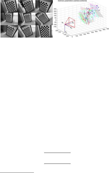
The iterative optimization in (2) above needs to be within the basin of convergence of the global minimum and so the linear method in (1) is used to determine an initial estimation of camera parameters. The raw data used as inputs to the process consists of the image corner positions, as detected by an automatic corner detector [18, 52], of all corners in all calibration images and the corresponding 2D world positions, [X, Y ]T , of the corners on the calibration grid. Typically, correspondences are established by manually clicking one or more detected image corners, and making a quick visual check that the imaged corners are matched correctly using overlaying graphics or text. A typical set of targets is shown in Fig. 2.6.

In the following four subsections we outline the theory and practice of camera calibration. The first subsection details the estimation of the planar projective mapping between a scene plane (calibration grid) and its image. The next two subsections closely follow Zhang [64] and detail the basic calibration and then the refined calibration, as outlined above. These subsections refer to the case of a single camera and so a final fourth subsection is used to describe the additional issues associated with the calibration of a stereo rig.

2.4.1 Estimation of a Scene-to-Image Planar Homography

A homography is a projective transformation (projectivity) that maps points to points and lines to lines. It is a highly useful imaging model when we view planar scenes,

50	S. Se and N. Pears

Fig. 2.6 Left: calibration targets used in a camera calibration process, image courtesy of Hao Sun. Right: after calibration, it is possible to determine the positions of the calibration planes using the estimated extrinsic parameters (Figure generated by the Camera Calibration Toolbox for Matlab, webpage maintained at Caltech by Jean-Yves Bouguet [9])

which is common in many computer vision processes, including the process of camera calibration.

Suppose that we view a planar scene, then we can define the (X, Y ) axes of the world coordinate system to be within the plane of the scene and hence Z = 0 everywhere. Equation (2.5) indicates that, as far as a planar scene is concerned, the imaging process can be reduced to:

λx = K[r1 r2 t][X, Y, 1]T ,

where r1 and r2 are the first and second columns of the rotation matrix R, hence:

λx = H[X, Y, 1]T ,

H = K[r1 r2 t].

(2.7)

The 3 × 3 matrix H is termed a planar homography, which is defined up to a scale factor,7 and hence has eight degrees of freedom instead of nine.

By expanding the above equation, we have:

	x h11				h12	h13 X					(2.8)
λ		y		h21	h22	h23		Y		.
		1		= h31	h32	h33		1

If we map homogeneous coordinates to inhomogeneous coordinates, by dividing through by λ, this gives:

x =

y =

h11X + h12Y + h13

h31X + h32Y + h33

h21X + h22Y + h23 .

h31X + h32Y + h33

(2.9)

(2.10)

7Due to the scale equivalence of homogeneous coordinates.

2 Passive 3D Imaging

51

From a set of four correspondences in a general position,8 we can formulate a set of eight linear equations in the eight unknowns of a homography matrix. This is because each correspondence provides a pair of constraints of the form given in Eqs. (2.9) and (2.10).

Rearranging terms in four pairs of those equations allows us to formulate the homography estimation problem in the form:

Ah = 0,

(2.11)

where A is an 8 × 9 data matrix derived from image and world coordinates of corresponding points and h is the 9-vector containing the elements of the homography matrix. Since A has rank 8, it has a 1-dimensional null space, which provides a non-trivial (non-zero vector) solution for Eq. (2.11). This can be determined from a Singular Value Decomposition (SVD) of the data matrix, which generates three matrices (U, D, V) such that A = UDVT . Here, D is a diagonal matrix of singular values and U, V are orthonormal matrices. Typically, SVD algorithms order the singular values in descending order down the diagonal of D and so the required solution, corresponding to a singular value of zero, is extracted as the last column of V. Due to the homogeneous form of Eq. (2.11), the solution is determined up to a nonzero scale factor, which is acceptable because H is only defined up to scale. Often a unit scale is chosen (i.e. h = 1) and this scaling is returned automatically in the columns of V.

In general, a larger number of correspondences than the minimum will not exactly satisfy the same homography because of image noise. In this case, a least squares solution to h can be determined in an over-determined system of linear equations. We follow the same procedure as above but this time the data matrix is of size 2n × 9 where n > 4 is the number of correspondences. When we apply SVD, we still select the last column of V corresponding to the smallest singular value in D. (Note that, in this case, the smallest singular value will be non-zero.)

Data normalization prior to the application of SVD is essential to give stable estimates [21]. The basic idea is to translate and scale both image and world coordinates to avoid orders of magnitude difference between the columns of the data matrix. Image points are translated so that their √centroid is at the origin and scaled to give a root-mean-squared (RMS) distance of 2 from that origin, so that the ‘average’ image point has coordinates of unity magnitude. Scene points should be normalized√ in a similar way except that they should be scaled to give an RMS distance of 3.

When using homogeneous coordinates, the normalizations can be applied using matrix operators Ni , Ns , such that new normalized coordinates are given as:

xn = Ni x, Xn = Ns X

for the image points and scene points respectively. Suppose that the homography

computed from normalized coordinates is ˜ , then the homography relating the orig-

H

inal coordinates of the correspondences is given as

	=	i ˜ s
H		N−1HN	.

8No three points collinear.