29.9. P, I, AND D RESPONSES GRAPHED

2311

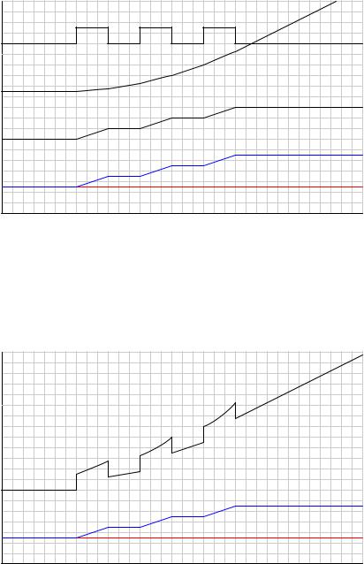
29.9.7Responses to a multiple ramps and steps

100
95	Derivative response
90
85
80
75
70	Integral response
65
60
55
% 50
45
40	Proportional response
35
30
25	PV
20
15	SP
10
5
0

Time

Proportional action directly mimics the ramp-and-step shape of the input. Integral action ramps slowly at first (when the error is small) but increases ramping rate as error increases. Which each higher ramp-and-step in PV, integral action winds up at an ever-increasing rate. Since PV never equals SP again, integral action never stops ramping upward. Derivative action steps with each ramp of the PV.

When combined into one PID output, the three actions produce this response:

	100
	95
	90
	85
	80
	75
	70
	65
	60	PID response
	55
	% 50
	45
	40
	35
	30
	25	PV
	20
	15	SP
	10
	5
	0

Time

2312	CHAPTER 29. CLOSED-LOOP CONTROL

29.9.8Responses to a sine wavelet

	100
	95
	90	Derivative response
	85
	80
	75
	70	Integral response
	65
	60
	55
	% 50
	45	Proportional response
	40
	35
	30	PV
	25
	20	SP
	15
	10
	5
	0
		Time

As always, proportional action directly mimics the shape of the input. The 90o phase shift seen in the integral and derivative responses, compared to the PV wavelet, is no accident or coincidence. The derivative of a sinusoidal function is always a cosine function, which is mathematically identical to a sine function with the angle advanced by 90o:

dxd (sin x) = cos x = sin(x + 90o)

Conversely, the integral of a sine function is always a negative cosine function14, which is mathematically identical to a sine function with the angle retarded by 90o:

Z

sin x dx = − cos x = sin(x − 90o)

In summary, the derivative operation always adds a positive (leading) phase shift to a sinusoidal input waveform, while the integral operation always adds a negative (lagging) phase shift to a sinusoidal input waveform.

14In this example, I have omitted the constant of integration (C) to keep things simple. The actual integral is as

R

such: sin x dx = −cos x + C = sin(x − 90o) + C. This constant value is essential to explaining why the integral response does not immediately “step” like the derivative response does at the beginning of the PV sine wavelet.

29.9. P, I, AND D RESPONSES GRAPHED

2313

When combined into one PID output, these particular integral and derivative actions mostly cancel, since they happen to be sinusoidal wavelets of equal amplitude and opposite phase. Thus, the only way that the final (PID) output di ers from proportional-only action in this particular case is the “steps” caused by derivative action responding to the input’s sudden rise at the beginning and end of the wavelet:

100
95
90
85
80
75
70
								PID			response
65
60
55
% 50
45
40
35
30
										PV
25
20
										SP
15
10
5
0
												Time

If the I and D tuning parameters were such that the integral and derivative responses were not equal in amplitude, their e ects would not completely cancel. Rather, the resultant of P, I, and D actions would be a sine wavelet having a phase shift somewhere between −90o and +90o exclusive, depending on the relative strengths of the P, I, and D actions.

The 90 degree phase shifts associated with the integral and derivative operations are useful to understand when tuning PID controllers. If one is familiar with these phase shift relationships, it is relatively easy to analyze the response of a PID controller to a sinusoidal input (such as when a process oscillates following a sudden load or setpoint change) to determine if the controller’s response is dominated by any one of the three actions. This may be helpful in “de-tuning” an over-tuned (overly aggressive) PID controller, if an excess of P, I, or D action may be identified from a phase comparison of PV and output waveforms.

2314	CHAPTER 29. CLOSED-LOOP CONTROL

29.9.9Note to students regarding quantitative graphing

A common exercise for students learning the function of PID controllers is to practice graphing a controller’s output given input (PV and SP) conditions, either qualitatively or quantitatively. This can be a frustrating experience for some students, as they struggle to accurately combine the e ects of P, I, and/or D responses into a single output trend. Here, I will present a way to ease the pain.

Suppose for example you were tasked with graphing the response of a PD (proportional + derivative) controller to the following PV and SP inputs over time. You are told the controller has a gain of 1, a derivative time constant of 0.3 minutes, and is reverse-acting:

	100
	95
	90
	85
	80
	75			PV
	70
	65
	60			SP
%	55
	50
	45	Output
	40
	35
	30
	25
	20
	15
	10
	5
	0
		0:15	0:30	0:45	1:00	1:15	1:30	1:45	2:00	2:15	2:30	2:45
					Time		(min:sec)

29.9. P, I, AND D RESPONSES GRAPHED

2315

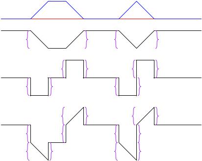
My first recommendation is to qualitatively sketch the individual P and D responses. Simply draw two di erent trends, each one right above or below the given PV/SP trends, showing the shapes of each response over time. You might even find it easier to do if you re-draw the original PV and SP trends on a piece of non-graph paper with the qualitative P and D trends also sketched on the same piece of non-graph paper. The purpose of the qualitative sketches is to separate the task of determining shapes from the task of determining numerical values, in order to simplify the process.

After sketching the separate P and D trends, label each one of the “features” (changes either up or down) in these qualitative trends. This will allow you to more easily combine the e ects into one output trend later:

P-only

D-only

PV

SP

P1

P2

P3

P4

	D3	D4	D7	D8
D1	D2		D5	D6

2316	CHAPTER 29. CLOSED-LOOP CONTROL

Now, you may qualitatively sketch an output trend combining each of these “features” into one graph. Be sure to label each ramp or step originating with the separate P or D trends, so you know where each “feature” of the combined output graph originates from:

P-only

D-only

P+D

PV

SP

P1

P2

P3

P4

	D3	D4	D7	D8
D1	D2		D5	D6

	P2	D4	P4	D8
D1	D3		D5	D7
P1	D2		P3	D6

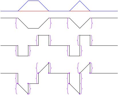
Once the general shape of the output has been qualitatively determined, you may go back to the separate P and D trends to calculate numerical values for each of the labeled “features.”

Note that each of the PV ramps is 15% in height, over a time of 15 seconds (one-quarter of a minute). With a controller gain of 1, the proportional response to each of these ramps will also be a ramp that is 15% in height.

Taking our given derivative time constant of 0.3 minutes and multiplying that by the PV’s rate-of-change ( dPVdt ) during each of its ramping periods (15% per one-quarter minute, or 60% per minute) yields a derivative response of 18% during each of the ramping periods. Thus, each derivative response “step” will be 18% in height.

29.9. P, I, AND D RESPONSES GRAPHED

2317

Going back to the qualitative sketches of P and D actions, and to the combined (qualitative) output sketch, we may apply the calculated values of 15% for each proportional ramp and 18% for each derivative step to the labeled “features.” We may also label the starting value of the output trend as given in the original problem (35%), to calculate actual output values at di erent points in time. Calculating output values at specific points in the graph becomes as easy as cumulatively adding and subtracting the P and D “feature” values to the starting output value:

PV

SP

P-only

D-only

P1		P2	P3		P4
15%		15%	15%		15%
	18%	18%		18%	18%
	D3	D4		D7	D8
D1	D2		D5		D6
18%	18%		18%		18%

53%

15% 18%

P2

D4

35%		18%	38%	35%
P+D
	D1	D3
	18%	17% 20%

53%

15% 18%

P4

D8

	38%	35%
D5		D7
18%	17%	18%

P1	D2	P3	D6
15%	18%	15%	18%
	2%		2%

2318	CHAPTER 29. CLOSED-LOOP CONTROL

Now that we know the output values at all the critical points, we may quantitatively sketch the output trend on the original graph:

	100
	95
	90
	85
	80
	75			PV
	70
	65
	60			SP
%	55
	50
	45	Output
	40
	35
	30
	25
	20
	15
	10
	5
	0
		0:15	0:30	0:45	1:00	1:15	1:30	1:45	2:00	2:15	2:30	2:45
					Time		(min:sec)

29.10Di erent PID equations

For better or worse, there are no fewer than three di erent forms of PID equations implemented in modern PID controllers: the parallel, ideal, and series. Some controllers o er the choice of more than one equation, while others implement just one. It should be noted that more variations of PID equation exist than these three, but that these are the three major variations.