9.3 Circular Motion

249

9.3 Circular Motion

How large forces acts on a roller coaster cart as it passes through a vertical loop, or on a car as it drives through a shape turn on the road? These are questions we can answer without having a specific model for the forces acting, because the motion is constrained: A roller coaster cart driving around a loop is constrained to follow the loop, since the cart is attached to the rail.

We have already seen how we can use constraints to find forces for linear motion. Fortunately, we can use exactly the same technique to determine the forces acting on an object following a curve. However, for curved motion we know that the acceleration also has a component normal to the curve: The centripetal acceleration. For curved motion we must therefore remember that even though the object follows a particular path, there must be a net force acting on the object in order for it to follow the path.

Linear and Curved Motion

We can illustrate the difference between linear and curved motion by looking at a bead moving along a wire, as illustrated in Fig. 9.12.

If the wire is shaped as a line, the bead can be accelerated along the wire but not normal to the wire. Hence, if we analyze the forces acting on the bead and apply Newton’s second law, we recognize that the net force in the x -direction along the

wire corresponds to

along the wire:

Fx = max .

(9.55)

Fig. 9.12 Left Illustration of a bead moving along a straight (linear) wire left and a circular (curved) wire (right)

250	9 Forces and Constrained Motion

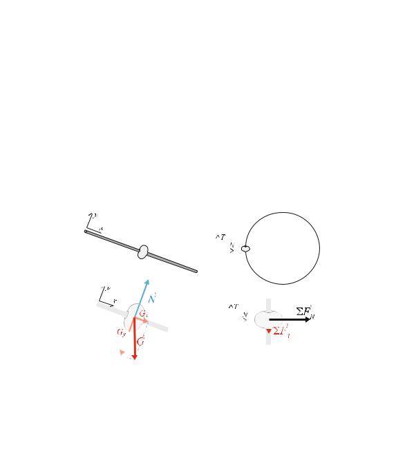
But in the direction normal to the wire (the y-direction), there is no motion and no acceleration. Therefore the net force is zero:

Fy = may = 0 .

(9.56)

If the wire is shaped as a circle, the analysis is different. Let us describe the motion of the bead using a coordinate system with one axis along the curve, the tangential axis, uˆ T ; and one axis normal to the curve pointing in towards the center of the circle, the normal axis, uˆ N . Again, we analyze the forces acting on the bead and apply Newton’s second law. The net force in the tangential direction is causing the tangential acceleration:

FT = maT ,

(9.57)

But in this case, the motion is not linear. Therefore, even though the bead follows the wire, it is accelerated also in the direction normal to the wire because the wire is curved. The net force in the normal direction is therefore related to the centripetal acceleration:

v2
FN = maN = m R .	(9.58)

This important difference between linear and curved motion is at the center of our analysis of curved constrained motion.

Structured Problem-Solving Approach

The method we apply when analyzing motion along a curved track consists of the following modification to the Model step in the structured problem-solving method:

•Find the forces acting on the object.

•Introduce models for the forces.

•In the normal direction the net force must produce the centripetal acceleration: aN = v2/R

•In the tangential direction the tangential acceleration is determined from the net tangential force.

You may then Solve to find the motion of the object and Analyze the solution to answer questions about the motion.

Types of Constraints

We can classify the constraints into two main types.

Non-conditional constraint: The constraint experienced by a bead moving along a wire. The bead follows the wire independently of the speed of the motion or any other property of the motion. Other similar cases are the motion of a weight attached to a rigid staff; the motion of a roller coaster car attached to a track; the motion of a

9.3 Circular Motion

251

person attached to a seat; or the motion of a train along a railway track. In the cases of a non-conditional constraint we can determine the forces and motion using the approach presented above.

Conditional constraint: The constraint experienced by a ball swung in a rope: As long as the rope is tight, the ball follows a circular path, because the rope pulls on the ball when stretched. But the rope does not exert any force when pushed. This means that the constraint in conditional: The ball is constrained to follow a circle only as long as the tensile force needed to make it follow a circle is positive. If the tensile force needed is negative, the rope cannot push the ball, and the constraint is no longer present. In this case the ball is only affected by gravity and air resistance until the rope is again tight. If you want to determine the motion of the ball when the rope is not tight, you apply Newton’s laws of motion to find the acceleration and solve to find the position and velocity of the ball using methods you are now proficient in.

Examples of Constrained Systems

A car on a hill-top: Usually we assume that a car driving along a bumpy road follows the vertical motion of the road. This is really a constraint on the motion: We assume that the car follows the path given by the road. If the car drives along a flat part of the road, this gives us a way to estimate the normal force. However, the normal force can only be positive: The car is not glued to the surface. The constraint on the motion of the car is therefore conditional: It can only follow the shape of the surface if this requires a positive normal force. If a negative normal force is required in order to follow the surface, the car looses contact with the surface.

A car driving through a curve: Usually, we assume that a car driving around a turn does not slide. The car therefore follows a specific track—the track given by the road. We can therefore analyze the motion of the car around a turn as if it was constrained—following a given curved track. This requires a net force on the car to give it the necessary centripetal acceleration. An important component in the net force is the friction force from the ground on the tires. But the friction force is limited by the maximum static friction force. Hence, the motion of the car is constrained to follow the curve, but only as long as the friction force is not exceeding its maximum.

9.3.1 Example: A Car Driving Through a Curve

Problem: A car is driving through a circular curve at constant speed. The coefficient of static friction between the tires of the car and the ground is µs . The speed of the car is v and the radius of the circle is R. How fast can the car drive before slipping?

Approach: This is an example of a conditional constrained problem: The car is constrained to follow a circular path, but only as long as the static friction force needed to give the car the required centripetal acceleration does not exceed the maximum frictional force.

252 9 Forces and Constrained Motion

(A)	(b)	N
	z
	Y
		fY
		G
		N
	Y
	z
	x
	x
	fx	G

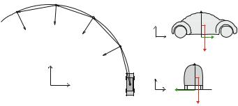
Fig. 9.13 a A car driving around a circular track. b Free-body diagram of the car

Identify: In this problem we address the motion of a car driving through a circular curve. We address the motion of the car as it passes the x -axis, as illustrated in Fig. 9.13. The motion of the car is in the x y-plane.

Model: The car is in contact with the road, giving rise to several contact forces: a normal force in the vertical direction, N , and a frictional force, f , from the ground on the car. The friction force has a component f y along the road and a component fx normal to the road (in the x -direction). In addition, the car is affected by the gravity,

G= mg in the z-direction. The free-body diagram of the car is shown in Fig. 9.13b. We relate the forces acting on the car to its acceleration by applying Newton’s

second law. The car is not moving in the vertical (z) direction, hence the acceleration az is zero:

Fz = N − G = N − mg = maz = 0 , (9.59)

The normal force from the ground on the car is therefore N = mg.

Because the car drives at constant speed, the acceleration in the tangential direction

along the road (the y-direction) is zero:
Fy = f y = may = 0 ,	(9.60)

Therefore the y-component of the friction force is zero.

Since the car follows a circular path, the car is accelerated in the normal direction, in toward the center of the circle. This corresponds to the −x direction in Fig. 9.13. Since the car is driving with a speed v, the normal acceleration corresponds to the

centripetal acceleration of an object moving in a circle of radius R:
Fx = fx = max = m −	v2	,	(9.61)
	R