76

Study of forced vibrations transition processes . . .

131

The use of devices called seismic insulating foundations involves the counteraction of building structures to seismic forces not by improving the strength properties of structures, but, as it is done in a wide variety of vibration protection systems, by reducing the seismic load on the protected objects. This is quite new for the earthquake-resistant constructing.

In work [1] we gave a review, a classification and the comparison of the devices designed to reduce the seismic load on buildings and which are the integral part of their foundations. Two classes of seismic isolating devices have been identified, which are the example of the direct transfer of vibro-isolation principles to constructing.

These are foundations with elastic support elements and dynamic dampers of seismic vibrations. Two classes of shock absorbers of a di erent kind have been established:

1.Foundations with servomechanisms, which include rigid supports with an indi erent or even unstable equilibrium position (balls, rollers, vertically arranged spars, etc.) and servomechanisms that return the building to its equilibrium position; at the same time, a compromise solution is often given, combining rolling or sliding bearings and elastic shock absorbers that replace servomechanisms;

2.Kinematic foundations, in which, as in foundations with servomechanisms, the seismic isolation is carried out not due to the elasticity of the shock absorber, but using supports of a special geometric shape; a building, a structure installed on such supports, has a stable equilibrium position, when removed from that position it oscillates with a frequency that depends [1,2] mainly on the geometric dimensions of the supports and the acceleration of gravity (for this reason, such devices are called kinematic [2] and [3] gravitational seismic isolation systems);

3.The most acceptable and promising from an engineering point of view, as noted in [1, 3], is the newest class of seismic isolating devices — a class of supporting kinematic foundations that favorably di er from other types of seismic shock absorbers in cost-e ectiveness and simplicity of technical solution.

The kinematic supports developed in connection with the requests of earthquake-resistant constructions can be used as shock absorbers in vibro-isolation systems of various machines and equipment, and as elements of devicesas well.

This article [19, 20] considers the oscillation of a solid body on kinematic foundations, the main elements of which are rolling bearers bounded by high-order surfaces of rotation at horizontal displacement of the foundation. Equations of motion of the vibro-protected body have been obtained. Stationary and transitional modes of the oscillatory process of the system have been investigated.

The work contains geometrical analysis of non-linear vibrations of vibro-protective systems on rolling bearers bearing elements of which are restricted by high order spherical surfaces in transition regime.

2 Literature review

Rolling bodies of various types are applied as the main element in many vibro-protective and seismo-protective devices.

The work [4] contains systematic depiction of non-linear systems analysis method, described by di erential equations of second rate. This work contains also topological and

132	Bissembayev K., Sultanova K.

graphical methods, applicable for calculation of autonomic and, especially, non-autonomic systems.

In the work [5] the author focuses attention on decision of tasks on determination of orders of initial conditions, leading to various stable stationary decisions. In the work [6] the author considers problems of self-oscillations of various mechanical systems, particularly, examines in detail self-oscillations of rotors.

The work [7] studies the features of vibrational motion of an orthogonal mechanism with disturbances, such as restricted power in the presence of a fixed load on the horizontal link. Dynamic and mathematical models were prepared, and the operating conditions’ fields of existence for the vibration mechanism in terms of the driving power were defined.

This paper [8] presents results of modelling of vibrations of rigid rotor caused by the degradation of hydrodynamic bearings. Model is composed applying equations of nonlinear hydrodynamic forces and measured parameters of a real rotary machine.

In order to study the resonance of a rotating circular plate under static loads in magnetic field, in the work [9] the nonlinear vibration equation about the spinning circular plate is derived according to Hamilton principle. The algebraic expression of the initial deflection and the magneto elastic forced disturbance di erential equation are obtained through the application of Galerkin integral method.

This paper [10] presents a new semi analytical approach for geometrically nonlinear vibration analysis of Euler-Bernoulli beams with di erent boundary conditions. The method makes use of Linstedt-Poincar’e perturbation technique to transform the nonlinear governing equations into a linear di erential equation system, whose solutions are then sought through the use of di erential quadrature approximation in space domain and an analytical series expansion in time domain.

In the work [11] a systematic method is developed for the dynamic analysis of the structures with sliding isolation which is a highly non-linear dynamic problem. According to the proposed method, a unified motion equation can be adapted for both stick and slip modes of the system. Unlike the traditional methods by which the integration interval has to be chopped into infinitesimal pieces during the transition of sliding and non-sliding modes, the integration interval remains constant throughout the whole process of the dynamic analysis by the proposed method so that accuracy and e ciency in the analysis of the non-linear system can be enhanced to a large extent.

The paper [12] features a survey of some recent developments in asymptotic techniques, which are valid not only for weakly nonlinear equations, but also for strongly ones. Further, the obtained approximate analytical solutions are valid for the whole solution domain. The limitations of traditional perturbation methods are illustrated, various modified perturbation techniques are proposed, and some mathematical tools such as variational theory, homotopy technology, and iteration technique are introduced to over-come the shortcomings.

The e ects of neglecting small harmonic terms on estimation of dynamical stability of the steady state solution determined in the frequency domain are considered in the paper[13]. For that purpose, a simple single-degree- of-freedom piecewise linear system excited by a harmonic excitation is analyzed. In the time domain, steady state solutions are obtained by using the method of piecing the exact solutions (MPES) and in the frequency domain, by the incremental harmonic balance method(IHBM). The stability of the solutions obtained in the frequency domain by IHBM is determined by using Floquet-Liapounov theorem and by

Study of forced vibrations transition processes . . .

133

digital simulation of the corresponding perturbed motion.

In the paper[14 ]the nonlinear response of a base-excited slender beam carrying an attached mass is investigated with 1:3:9 internal resonances for principal and combination parametric resonances.

3 Material and methods

3.1 Equations of the motion

Let us consider the principle of work of the kinematic foundation of moving supporting elements, which is a rolling bearing with bounded surfaces of rotation of a high (n) order (Fig.1).

On the Figure 1, the object I is a rolling bearing with bounded (top and bottom) surfaces of rotation, expressed by formulas

y1 = a1x1n, y2 = a2x1m

(1)

and having a common axis of symmetry; but objects 2 and 3 are stationary base (foundation) and inner coat of the vibro-protected body.

Equations (1) are referred to the coordinate system associated with the rolling bearings (See Fig.1). The curvature radius of the vertices of these surfaces at n, m > 2 tends to infinity, i.e. there is straightening of the bearing surfaces. Let us denote the horizontal o set of the bases as x˜0(t). As x˜(t) we denote a displacement of the upper body, supporting on the rolling bearing.

Figure 1: Scheme of rolling bearingswith higher ordersurfaces
The equation (2) can be reduced to an equation in dimensionless form [19]:
x¨ + Φ(x − x0) − x = −x0(t),			(2)
where
1
Φ(x − x0) = Nn(x − x0)n − 1 ,			(3)

134	Bissembayev K., Sultanova K.

Nn =	1			1				+	1			).	(4)
				(
	1				n 1
									n 1
	n−√nH				−√a1				−√a2

3.2 Periodic solutions and their stability

Let us study the vibrations of a body at harmonic horizontal displacement of the lower base

x0(t) = Q sin pt,

(5)

where Q and p – dimensionless amplitude and frequency of perturbations.

Assuming that in the case of harmonic oscillations, a component of the fundamental frequency, having period 2π/p, dominates over the higher harmonics. Periodic solution and first derivative of the equation (5) can be approximately represented as,

x = a sin pt + b cos pt, x˙ = ap cos pt − bp sin pt,

(6)

Let us suppose that the amplitudes a and b are functions of time and slowly vary depending on t.

For the nonlinear term of the equation (2), Fourier series expansion looks as:

1

1

∞

k

Φ(x−x0) = NnC n − 1 sinn − 1 (pt+γ) =

=1

B2k−1 sin(2k−1)pt+D2k−1 cos(2k−1)pt, (7)

where

n − 2

−

a − Q

2k−1

n

2k−1 [(a − Q)2 + b2]

−

(8)

b

(a − Q)

2(n

1)

C =

(a

Q)2

+ b2, tgγ =

,

B

= N

K

,

D2k−1 = NnK2k−1

n − 2 , K2k−1 = (L22k−1 + M22k−1,

b

[(a − Q)2 + b2]2(n − 1)

1

2π

1

1

2π

1

0

sinn

− 1

ψ sin(2k−1)ψdψ, M2k−1 =

0 sinn − 1 ψ cos(2k−1)ψdψ, ψ = pt+γ.

L2k−1 =

π

π

Substituting (6), (7) to (2) and equating to zero the individual coe cients of the terms,

containing sin pt and cos pt, we have

da

1

2

1

=

(p

+ 1)

−

NnK1

b = X(a, b),

dt

p

−

[(a − Q)2 + b2]2(n − 1)

Study of forced vibrations transition processes . . .

135

db

1

2

1

2

=

(p

+ 1)

NnK1

(a

−

Q) + p

Q

= Y (a, b). (9)

dt

−p

−

−

[(a

−

Q)

+ b

]

−

Let us consider the steady state, when amplitudes a(t) and b(t) in (6) are constant, i.e.
	da		= X(a, b) = 0,	db	= Y (a, b) = 0.	(10)
	dt			dt

In light of these conditions, from equations (9) we can get that the set amplitude a0 = A,

b0 = 0 of the periodic solution x(t) is determined by the formula
A = p2 + 1		NnK1(A		Q)n − 1	+ Q .	(11)
1				1
			−

Let us derive the conditions for the stability of periodic solutions. We will consider small deviations ξ and η from the amplitudes a0 and b0 and will find out, when these deviations (with increasing time) are close to zero.

From equation (9) we get

dξ

= α1ξ

+ α2η,

dt

(12)

dη

= β1ξ

+ β2η,

dt

Where

α

=

(n − 2)

1

W0

(a

Q)b

,

1

(n

−

1) p C2

0 −

0

0

(n − 1) C02 0:

p 4

−

α2 =

1

(p2 + 1)

W0 +

(n

− 2)

W0

b2 ,

(13)

p 4−

−

n − 1 C02

−

:

β1 =

1

(p2 + 1) + W0

(

n

−

2

)

W0

(a0

Q)2 ,

−p 4 n − 1 C02

−

:

β2 =

1

(

n −

2

)

W0

(a0

Q)b0

,

where

W0 =

NnK1

, C0

= A − Q.

n − 2

C0n − 1

136	Bissembayev K., Sultanova K.

The characteristic equation of the system has the form:

λ2 − (α1 + β2)λ + α1β2 − α2β1 = 0.

(14)

The stability condition is given by Routh-Hurwitz criteria, i.e.

		α1 + β2 = 0, (α1 = 0, β2 = 0).
to			α1β2 − α2β1 > 0
(p2	+ 1) − W0	8(p2 + 1) −	W0	9 > 0.	(15)
			n 1
5	6		−

The singular point, i.e. steady system state, is a center.

The boundary of unstable periodic solutions of equations (9) is determined by the curves.

p2 = W0 − 1,	p2 =	W0							(16)
				− 1
		n − 1
and stability areas are determined by the following inequalities [19]
p2 − (W0 − 1)	> 0, p2 − (			W0			− 1) > 0,
				n − 1					(17)
p2 − (W0 − 1)	< 0, p2 − (				W0			− 1) < 0.
					n − 1

4 Simulation Results:Geometric analysis of the integral curves

From equation (9), we have

Y (a, b)da − X(a, b)db = 0.

(18)

As due to equations (9) ∂X∂a + ∂Y∂b = 0, the equation (9) becomes integrable, and its complete integral has the form

C2

2(n − 1)

n

−

(p2

+ 1)

+

N

K

C n

−

1

−

p2Qa = E,

(19)

n

2

n

1

where E – constant of integration. In order to examine the integral curves in the neighborhood of a singular point, we move the origin of coordinates to this particular point a0, b0 introducing new variables ξ and η, namely:

a = a0 + ξ, b = b0 + η.

Study of forced vibrations transition processes . . .

137

Then the basic system of equations (9) takes the form,

9 C02

dt

n − 1 p

82

−

2

2

2

dξ

= α1

ξ + α2η + (

n − 2

)

1

1

b0ξ2

+ (a0

Q)ξη +

3

b0

η2

+

1

ξ2η +

1

η3

W0

,

82

9 C02

(20)

dt

n − 1 p

−

2

−

2

2

dη

= β1

ξ + β2η + (

n − 2

)

1

3

(a0

Q)ξ2 + b0ξη +

1

(a0

Q)η2 +

1

ξη2

+

1

ξ3

W0

,

where the following relations are used

9

−

n − 1 C02

8

−

2

2

n − 2

n − 2

W = W0

(

n − 2

)

W0

(a0

Q)ξ +

1

ξ2 + b0η +

1

η2 , W =

NnK1

, W0 =

NnK1

C n − 1

C0n − 1

Taking into account that b0 = 0due to the equation (9), we get

dt = α¯2

η + (n −−

1)p

n

3n − 4 8(a0

− Q)ξη + 2ξ2

η +

2η39

,

dξ

n

2 1

N

K1

1

1

(a0 − Q) n − 1

82(a0 − Q)ξ2 + 2(a0 − Q)η2 + 2ξη2 +

2ξ39,

(21)

dt = β¯1

ξ + (n −−

1)p

n

3n − 4

dη

n

2 1

N

K1

3

1

1

1

(a0 − Q) n − 1

where

α¯2 =

1

(p2 + 1)

NnK1

, β¯1

=

1

(p2 + 1)

NnK1

.

−

n − 2

p

−

n − 2

p

−

(a0

(n

1)(a0

−

−

−

−

−

Equations (21) are integrated. As a result of integration we obtain

β¯1ξ2 − α¯2η2 + (n −−

1)p

n

3n − 4

8(a0 − Q)ξ3 + 4(ξ4 − η4)9

= F,

(22)

n

2

1

N

K1

1

(a0 − Q) n − 1

where F – constant of integration.

In order to classify the type of singular points, we calculate the roots of the characteristic

equation (14):

λ1,2

=

1

2

±

2−

β2)2

2

1

,

α

+ β

(α1

+ 4α

β

where from

138 Bissembayev K., Sultanova K.

λ1, λ2 = ± α2β1, α1 + β2 = 0.

The dependence curve between Q and A0 is presented on Fig. 2. Let us divide the curve into three parts 1, 2, 3 (as shown in Fig. 2): the boundaries of each part are determined by the points D and B, for which,

=

			A =	NnK1 n−2
				p2 + 1
A =	[(n − 1)(p2 + 1) − 1]					·
	(n	−	1)(p2 + 1)p2

	NnK1			,
	p2 + 1
n−=2					NnK1		.
			(n	−	1)(p2	+ 1)

These areas correspond to the following special terms:

1.Center (α2β1 < 0)

2.Saddle (α2β1 > 0)

3.Center (α2β1 < 0)

We shall consider the case when Q = 0.014081. Here there are three possible states of equilibrium (Fig. 2); data for the respective singular points are shownin Table 1.

Table 1. – Singular points (Fig. 3)

Singular	A0	λ1, λ2	μ1, μ2	Classification
point
1	-0.055919	±1.209i		Center
2	0.045107	1.552	1.139	Saddle
3	0.015344	±18.965i		Center

Directions of the integral curves at the singular points (node and saddle) can be found by the following expression

μ1,2 = −(α1 − β2) ± (α1 − β2)2 + 4α2β1 .

2α2

Integral curves of equation (9) can be easily obtained by using equation (19) for di erent values of E. The results are shown in Fig. 3. We see that in a conservative system, each integral curve forms a closed trajectory, which does not tend to a stable singular point.

This means that the amplitude and phase fluctuations angle in a steady state do not remain constant, but vary periodically. Thus the phase fluctuations can outperform an external force and be behind it. If a closed trajectory does not cover the origin of coordinates, so the angle of advance and the angle of retard are mutually compensated after passing the representation point over a closed trajectory, and an oscillation will be synchronized with an external force. On the other hand, if the origin of coordinates is located inside a closed trajectory, so as a result of each cycle, there will be a phase di erence of 2π radian, and oscillation will not be synchronized with the external force.

a. The integral curves of the system, corresponding to the point D (Fig. 2).

Assuming that Q = 0 in equations (9), we have

dadb = −ab

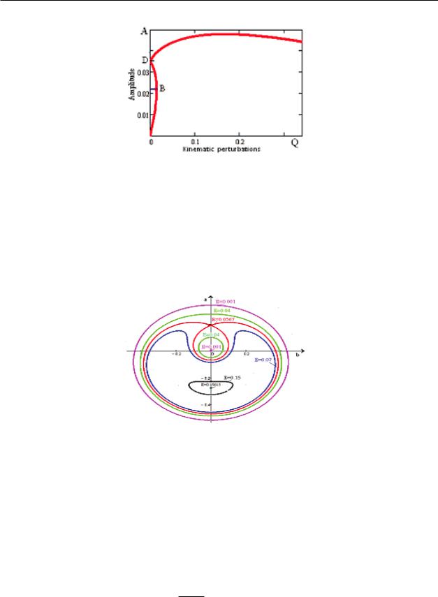
Study of forced vibrations transition processes . . .

139

Figure 2: Amplitude response curve for harmonic vibration

or after integration

a2 + b2 = const.

Consequently, the integral curves form a family of concentric circles with a center at the coordinate origin, so that the singular point (in this case - the origin of coordinates) is a center.

Figure 3: Cumulative curves for harmonic vibration

Period T , necessary in order to the representation points a(t) and b(t) make one revolution along a closed trajectory, is defined by the expression.

T = >	X2(a, b) + Y 2			(a, b)	= >		[p2 − (W − 1)] A		= p2 − (W − 1),	(23)
		ds						pds	2πp
ds = (da)2 + (db)2, W =						nn−12 .
						N K

An − 1

Now let us suppose, that the initial condition is given by the point a(0), b(0) located on a

140	Bissembayev K., Sultanova K.

n − 1

circle of radius A = ( NnK1 )n − 2 ; then the period T will be equal to infinity. As can be p2 + 1

seen from the equations (9), the representation point a(t), b(t) in this case remains in its initial position. This means that the oscillation frequency coincides with the frequency of the

external forces. Then from equations (9) we can see that the representation point a(t), b(t) n − 1

is moving circumferentially in the counterclockwise direction when A > ( NnK1 )n − 2 , and p2 + 1

n − 1

in the clockwise direction – when A < ( NnK1 )n − 2 . p2 + 1

In the first case, the oscillation frequency is higher than the external force; in the second case, the pattern will be reversed. So we can conclude, that the oscillation frequency varies depending on A and coincides with the frequency of an external force only in the case where

n − 1

A = ( NnK1 )n − 2 . p2 + 1

b. The integral curves of the system, corresponding to the point B (Fig. 2)

In this case, from equations (11), we obtain

(n

1)(p2 + 1)

NnK1

n − 1

Q =

−

8

9n − 2

, b0 = 0,

p2

(n − 1)(p2 + 1)

n − 1

(24)

n(p2 + 1)

1

NnK1

a0 = A =

−

·

8

9n − 2 .

p2

(n − 1)(p2 + 1)

Let us investigate nature of the singular point B. From (21) we have

α¯2 = −(n − 2)

p2 + 1

¯

= 0,

p

, β1

Where from λ1 = λ2 = 0. Then equation (21) takes the form

dξdt = −γη + C1(C0ξη + 12ξ2η + 12η3),

(25)

dηdt = 12C1(3C0ξ2 + C0η2 + ξη2 + ξ3),

Where

																3n − 4
γ = (n	−	2)	p2 + 1	,	C		=	1	(	n −		2	)	[(n − 1)(p2 + 1)] n − 2				,
			p			1						1
								p n			−			(N K	)2		(26)
														n 1

89

C0 =	NnK1
		.
	(n − 1)(p2 + 1)