

- •About the author
- •Brief Contents
- •Contents
- •Preface
- •This Book’s Approach
- •What’s New in the Seventh Edition?
- •The Arrangement of Topics
- •Part One, Introduction
- •Part Two, Classical Theory: The Economy in the Long Run
- •Part Three, Growth Theory: The Economy in the Very Long Run
- •Part Four, Business Cycle Theory: The Economy in the Short Run
- •Part Five, Macroeconomic Policy Debates
- •Part Six, More on the Microeconomics Behind Macroeconomics
- •Epilogue
- •Alternative Routes Through the Text
- •Learning Tools
- •Case Studies
- •FYI Boxes
- •Graphs
- •Mathematical Notes
- •Chapter Summaries
- •Key Concepts
- •Questions for Review
- •Problems and Applications
- •Chapter Appendices
- •Glossary
- •Translations
- •Acknowledgments
- •Supplements and Media
- •For Instructors
- •Instructor’s Resources
- •Solutions Manual
- •Test Bank
- •PowerPoint Slides
- •For Students
- •Student Guide and Workbook
- •Online Offerings
- •EconPortal, Available Spring 2010
- •eBook
- •WebCT
- •BlackBoard
- •Additional Offerings
- •i-clicker
- •The Wall Street Journal Edition
- •Financial Times Edition
- •Dismal Scientist
- •1-1: What Macroeconomists Study
- •1-2: How Economists Think
- •Theory as Model Building
- •The Use of Multiple Models
- •Prices: Flexible Versus Sticky
- •Microeconomic Thinking and Macroeconomic Models
- •1-3: How This Book Proceeds
- •Income, Expenditure, and the Circular Flow
- •Rules for Computing GDP
- •Real GDP Versus Nominal GDP
- •The GDP Deflator
- •Chain-Weighted Measures of Real GDP
- •The Components of Expenditure
- •Other Measures of Income
- •Seasonal Adjustment
- •The Price of a Basket of Goods
- •The CPI Versus the GDP Deflator
- •The Household Survey
- •The Establishment Survey
- •The Factors of Production
- •The Production Function
- •The Supply of Goods and Services
- •3-2: How Is National Income Distributed to the Factors of Production?
- •Factor Prices
- •The Decisions Facing the Competitive Firm
- •The Firm’s Demand for Factors
- •The Division of National Income
- •The Cobb–Douglas Production Function
- •Consumption
- •Investment
- •Government Purchases
- •Changes in Saving: The Effects of Fiscal Policy
- •Changes in Investment Demand
- •3-5: Conclusion
- •4-1: What Is Money?
- •The Functions of Money
- •The Types of Money
- •The Development of Fiat Money
- •How the Quantity of Money Is Controlled
- •How the Quantity of Money Is Measured
- •4-2: The Quantity Theory of Money
- •Transactions and the Quantity Equation
- •From Transactions to Income
- •The Assumption of Constant Velocity
- •Money, Prices, and Inflation
- •4-4: Inflation and Interest Rates
- •Two Interest Rates: Real and Nominal
- •The Fisher Effect
- •Two Real Interest Rates: Ex Ante and Ex Post
- •The Cost of Holding Money
- •Future Money and Current Prices
- •4-6: The Social Costs of Inflation
- •The Layman’s View and the Classical Response
- •The Costs of Expected Inflation
- •The Costs of Unexpected Inflation
- •One Benefit of Inflation
- •4-7: Hyperinflation
- •The Costs of Hyperinflation
- •The Causes of Hyperinflation
- •4-8: Conclusion: The Classical Dichotomy
- •The Role of Net Exports
- •International Capital Flows and the Trade Balance
- •International Flows of Goods and Capital: An Example
- •Capital Mobility and the World Interest Rate
- •Why Assume a Small Open Economy?
- •The Model
- •How Policies Influence the Trade Balance
- •Evaluating Economic Policy
- •Nominal and Real Exchange Rates
- •The Real Exchange Rate and the Trade Balance
- •The Determinants of the Real Exchange Rate
- •How Policies Influence the Real Exchange Rate
- •The Effects of Trade Policies
- •The Special Case of Purchasing-Power Parity
- •Net Capital Outflow
- •The Model
- •Policies in the Large Open Economy
- •Conclusion
- •Causes of Frictional Unemployment
- •Public Policy and Frictional Unemployment
- •Minimum-Wage Laws
- •Unions and Collective Bargaining
- •Efficiency Wages
- •The Duration of Unemployment
- •Trends in Unemployment
- •Transitions Into and Out of the Labor Force
- •6-5: Labor-Market Experience: Europe
- •The Rise in European Unemployment
- •Unemployment Variation Within Europe
- •The Rise of European Leisure
- •6-6: Conclusion
- •7-1: The Accumulation of Capital
- •The Supply and Demand for Goods
- •Growth in the Capital Stock and the Steady State
- •Approaching the Steady State: A Numerical Example
- •How Saving Affects Growth
- •7-2: The Golden Rule Level of Capital
- •Comparing Steady States
- •The Transition to the Golden Rule Steady State
- •7-3: Population Growth
- •The Steady State With Population Growth
- •The Effects of Population Growth
- •Alternative Perspectives on Population Growth
- •7-4: Conclusion
- •The Efficiency of Labor
- •The Steady State With Technological Progress
- •The Effects of Technological Progress
- •Balanced Growth
- •Convergence
- •Factor Accumulation Versus Production Efficiency
- •8-3: Policies to Promote Growth
- •Evaluating the Rate of Saving
- •Changing the Rate of Saving
- •Allocating the Economy’s Investment
- •Establishing the Right Institutions
- •Encouraging Technological Progress
- •The Basic Model
- •A Two-Sector Model
- •The Microeconomics of Research and Development
- •The Process of Creative Destruction
- •8-5: Conclusion
- •Increases in the Factors of Production
- •Technological Progress
- •The Sources of Growth in the United States
- •The Solow Residual in the Short Run
- •9-1: The Facts About the Business Cycle
- •GDP and Its Components
- •Unemployment and Okun’s Law
- •Leading Economic Indicators
- •9-2: Time Horizons in Macroeconomics
- •How the Short Run and Long Run Differ
- •9-3: Aggregate Demand
- •The Quantity Equation as Aggregate Demand
- •Why the Aggregate Demand Curve Slopes Downward
- •Shifts in the Aggregate Demand Curve
- •9-4: Aggregate Supply
- •The Long Run: The Vertical Aggregate Supply Curve
- •From the Short Run to the Long Run
- •9-5: Stabilization Policy
- •Shocks to Aggregate Demand
- •Shocks to Aggregate Supply
- •10-1: The Goods Market and the IS Curve
- •The Keynesian Cross
- •The Interest Rate, Investment, and the IS Curve
- •How Fiscal Policy Shifts the IS Curve
- •10-2: The Money Market and the LM Curve
- •The Theory of Liquidity Preference
- •Income, Money Demand, and the LM Curve
- •How Monetary Policy Shifts the LM Curve
- •Shocks in the IS–LM Model
- •From the IS–LM Model to the Aggregate Demand Curve
- •The IS–LM Model in the Short Run and Long Run
- •11-3: The Great Depression
- •The Spending Hypothesis: Shocks to the IS Curve
- •The Money Hypothesis: A Shock to the LM Curve
- •Could the Depression Happen Again?
- •11-4: Conclusion
- •12-1: The Mundell–Fleming Model
- •The Goods Market and the IS* Curve
- •The Money Market and the LM* Curve
- •Putting the Pieces Together
- •Fiscal Policy
- •Monetary Policy
- •Trade Policy
- •How a Fixed-Exchange-Rate System Works
- •Fiscal Policy
- •Monetary Policy
- •Trade Policy
- •Policy in the Mundell–Fleming Model: A Summary
- •12-4: Interest Rate Differentials
- •Country Risk and Exchange-Rate Expectations
- •Differentials in the Mundell–Fleming Model
- •Pros and Cons of Different Exchange-Rate Systems
- •The Impossible Trinity
- •12-6: From the Short Run to the Long Run: The Mundell–Fleming Model With a Changing Price Level
- •12-7: A Concluding Reminder
- •Fiscal Policy
- •Monetary Policy
- •A Rule of Thumb
- •The Sticky-Price Model
- •Implications
- •Adaptive Expectations and Inflation Inertia
- •Two Causes of Rising and Falling Inflation
- •Disinflation and the Sacrifice Ratio
- •13-3: Conclusion
- •14-1: Elements of the Model
- •Output: The Demand for Goods and Services
- •The Real Interest Rate: The Fisher Equation
- •Inflation: The Phillips Curve
- •Expected Inflation: Adaptive Expectations
- •The Nominal Interest Rate: The Monetary-Policy Rule
- •14-2: Solving the Model
- •The Long-Run Equilibrium
- •The Dynamic Aggregate Supply Curve
- •The Dynamic Aggregate Demand Curve
- •The Short-Run Equilibrium
- •14-3: Using the Model
- •Long-Run Growth
- •A Shock to Aggregate Supply
- •A Shock to Aggregate Demand
- •A Shift in Monetary Policy
- •The Taylor Principle
- •14-5: Conclusion: Toward DSGE Models
- •15-1: Should Policy Be Active or Passive?
- •Lags in the Implementation and Effects of Policies
- •The Difficult Job of Economic Forecasting
- •Ignorance, Expectations, and the Lucas Critique
- •The Historical Record
- •Distrust of Policymakers and the Political Process
- •The Time Inconsistency of Discretionary Policy
- •Rules for Monetary Policy
- •16-1: The Size of the Government Debt
- •16-2: Problems in Measurement
- •Measurement Problem 1: Inflation
- •Measurement Problem 2: Capital Assets
- •Measurement Problem 3: Uncounted Liabilities
- •Measurement Problem 4: The Business Cycle
- •Summing Up
- •The Basic Logic of Ricardian Equivalence
- •Consumers and Future Taxes
- •Making a Choice
- •16-5: Other Perspectives on Government Debt
- •Balanced Budgets Versus Optimal Fiscal Policy
- •Fiscal Effects on Monetary Policy
- •Debt and the Political Process
- •International Dimensions
- •16-6: Conclusion
- •Keynes’s Conjectures
- •The Early Empirical Successes
- •The Intertemporal Budget Constraint
- •Consumer Preferences
- •Optimization
- •How Changes in Income Affect Consumption
- •Constraints on Borrowing
- •The Hypothesis
- •Implications
- •The Hypothesis
- •Implications
- •The Hypothesis
- •Implications
- •17-7: Conclusion
- •18-1: Business Fixed Investment
- •The Rental Price of Capital
- •The Cost of Capital
- •The Determinants of Investment
- •Taxes and Investment
- •The Stock Market and Tobin’s q
- •Financing Constraints
- •Banking Crises and Credit Crunches
- •18-2: Residential Investment
- •The Stock Equilibrium and the Flow Supply
- •Changes in Housing Demand
- •18-3: Inventory Investment
- •Reasons for Holding Inventories
- •18-4: Conclusion
- •19-1: Money Supply
- •100-Percent-Reserve Banking
- •Fractional-Reserve Banking
- •A Model of the Money Supply
- •The Three Instruments of Monetary Policy
- •Bank Capital, Leverage, and Capital Requirements
- •19-2: Money Demand
- •Portfolio Theories of Money Demand
- •Transactions Theories of Money Demand
- •The Baumol–Tobin Model of Cash Management
- •19-3 Conclusion
- •Lesson 2: In the short run, aggregate demand influences the amount of goods and services that a country produces.
- •Question 1: How should policymakers try to promote growth in the economy’s natural level of output?
- •Question 2: Should policymakers try to stabilize the economy?
- •Question 3: How costly is inflation, and how costly is reducing inflation?
- •Question 4: How big a problem are government budget deficits?
- •Conclusion
- •Glossary
- •Index

468 | P A R T V Macroeconomic Policy Debates
economists. According to the Ricardian view, government debt does not influence national saving and capital accumulation. As we will see, the debate between the traditional and Ricardian views of government debt arises from disagreements over how consumers respond to the government’s debt policy.
Section 16-5 then looks at other facets of the debate over government debt. It begins by discussing whether the government should always try to balance its budget and, if not, when a budget deficit or surplus is desirable. It also examines the effects of government debt on monetary policy, the political process, and a nation’s role in the world economy.
16-1 The Size of the Government Debt
Let’s begin by putting the government debt in perspective. In 2008, the debt of the U.S. federal government was $5.8 trillion. If we divide this number by 305 million, the number of people in the United States, we find that each person’s share of the government debt was about $19,000. Obviously, this is not a trivial number—few people sneeze at $19,000. Yet if we compare this debt to the roughly $1.5 million a typical person will earn over his or her working life, the government debt does not look like the catastrophe it is sometimes made out to be.
One way to judge the size of a government’s debt is to compare it to the amount of debt other countries have accumulated. Table 16-1 shows the
TA B L E 16-1
How Indebted Are the World’s Governments?
|
Government Debt as |
|
Government Debt as |
Country |
a Percentage of GDP |
Country |
a Percentage of GDP |
|
|
|
|
Japan |
173.0 |
Switzerland |
48.1 |
Italy |
113.0 |
Norway |
45.4 |
Greece |
100.8 |
Sweden |
44.6 |
Belgium |
92.2 |
Spain |
44.2 |
United States |
73.2 |
Finland |
39.6 |
France |
72.5 |
Slovak Republic |
38.0 |
Hungary |
71.8 |
Czech Republic |
36.1 |
Portugal |
70.9 |
Ireland |
32.8 |
Germany |
64.8 |
Korea |
32.6 |
Canada |
63.0 |
Denmark |
28.4 |
Austria |
62.6 |
New Zealand |
25.3 |
United Kingdom |
58.7 |
Iceland |
24.8 |
Netherlands |
54.5 |
Luxembourg |
18.1 |
Poland |
52.8 |
Australia |
14.2 |
Source: OECD Economic Outlook. Data are based on estimates of gross government financial liabilities and nominal GDP for 2008.
C H A P T E R 1 6 Government Debt and Budget Deficits | 469
amount of government debt for 28 major countries expressed as a percentage of each country’s GDP. At the top of the list are the heavily indebted countries of Japan and Italy, which have accumulated a debt that exceeds annual GDP. At the bottom are Luxembourg and Australia, which have accumulated relatively small debts. The United States is not far from the middle of the pack. By international standards, the U.S. government is neither especially profligate nor especially frugal.
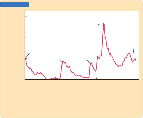
Over the course of U.S. history, the indebtedness of the federal government has varied substantially. Figure 16-1 shows the ratio of the federal debt to GDP since 1791. The government debt, relative to the size of the economy, varies from close to zero in the 1830s to a maximum of 107 percent of GDP in 1945.
Historically, the primary cause of increases in the government debt is war. The debt–GDP ratio rises sharply during major wars and falls slowly during peacetime. Many economists think that this historical pattern is the appropriate way to run fiscal policy. As we will discuss more fully later in this chapter, deficit financing of wars appears optimal for reasons of both tax smoothing and generational equity.
FIGURE 16-1
Debt–GDP ratio
1.2
World War II
1 |
|
|
|
|
|
|
|
|
|
|
|
0.8 |
|
|
|
|
|
|
|
|
|
|
|
0.6 |
Revolutionary |
|
|
|
|
|
|
|
Iraq War |
||
|
|
|
|
|
|
|
|
|
|||
|
|
|
|
|
|
|
|
|
|
||
|
War |
|
Civil |
|
|
|
|
|
|
|
|
|
|
|
|
|
|
|
|
|
|
|
|
0.4 |
|
|
War |
|
World War I |
|
|
|
|
|
|
0.2 |
|
|
|
|
|
|
|
|
|
|
|
0 |
1811 |
1831 |
1851 |
1871 |
1891 |
1911 |
1931 |
1951 |
1971 |
1991 |
2008 |
1791 |
|||||||||||
Year
The Ratio of Government Debt to GDP Since 1790 The U.S. federal government debt held by the public, relative to the size of the U.S. economy, rises sharply during wars and declines slowly during peacetime. A major exception is the period from 1980 to 1995, when the ratio of debt to GDP rose without the occurrence of a major military conflict.
Source: U.S. Department of the Treasury, U.S. Department of Commerce, and T. S. Berry, “Production and Population Since 1789,” Bostwick Paper No. 6, Richmond, 1988.

470 | P A R T V Macroeconomic Policy Debates
One instance of a large increase in government debt in peacetime began in the early 1980s. When Ronald Reagan was elected president in 1980, he was committed to reducing taxes and increasing military spending. These policies, coupled with a deep recession attributable to tight monetary policy, began a long period of substantial budget deficits. The government debt expressed as a percentage of GDP roughly doubled from 26 percent in 1980 to 50 percent in 1995. The United States had never before experienced such a large increase in government debt during a period of peace and prosperity. Many economists have criticized this increase in government debt as imposing an unjustifiable burden on future generations.
The increase in government debt during the 1980s caused significant concern among many policymakers as well. The first President Bush raised taxes to reduce the deficit, breaking his “Read my lips: No new taxes” campaign pledge and, according to some political commentators, costing him reelection. In 1993, when President Clinton took office, he raised taxes yet again. These tax increases, together with spending restraint and rapid economic growth due to the infor- mation-technology boom, caused the budget deficits to shrink and eventually turn into budget surpluses. The government debt fell from 50 percent of GDP in 1995 to 33 percent in 2001.
When President George W. Bush took office in 2001, the high-tech boom in the stock market was reversing course, and the economy was heading into recession. Economic downturns automatically cause tax revenue to fall and push the budget toward deficit. In addition, tax cuts to combat the recession and increased spending for homeland security and wars in Afghanistan and Iraq further increased the budget deficit, which averaged about 3 percent of GDP during his tenure. From 2001 to 2008, government debt rose from 33 to 41 percent of GDP.
When President Barack Obama moved into the White House in 2009, the economy was in the midst of a deep recession. Tax revenues were declining as the economy shrank. In addition, one of the new president’s first actions was to sign a large fiscal stimulus to prop up the aggregate demand for goods and services. (A Case Study in Chapter 10 examines this policy.) The federal government’s budget deficit was projected to be 12 percent of GDP in 2009 and 8 percent in 2010—levels not experienced since World War II. The debt–GDP ratio was projected to continue rising, at least in the near term.
In his first budget proposal, President Obama proposed reducing the budget deficit over time to 3 percent of GDP in 2013. The success of this initiative remained to be seen as this book went to press. Regardless, these events ensured that the economic effects of government debt would remain a major policy concern in the years to come.
CASE STUDY
The Troubling Long-Term Outlook for Fiscal Policy
What does the future hold for fiscal policymakers? Economic forecasting is far from precise, and it is easy to be cynical about economic predictions. But good policy cannot be made if policymakers only look backward. As a result,
C H A P T E R 1 6 Government Debt and Budget Deficits | 471
economists in the Congressional Budget Office (CBO) and other government agencies are always trying to look ahead to see what problems and opportunities are likely to develop. When these economists conduct long-term projections of U.S. fiscal policy, they paint a troubling picture.
One reason is demographic. Advances in medical technology have been increasing life expectancy, while improvements in birth-control techniques and changing social norms have reduced the number of children people have. Because of these developments, the elderly are becoming a larger share of the population. In 1950, the elderly population (aged 65 and older) made up about 14 percent of the working-age population (aged 20 to 64). Now the elderly are about 21 percent of the working-age population, and that figure will rise to about 40 percent in 2050. About one-third of the federal budget is devoted to providing the elderly with pensions (mainly through the Social Security program) and health care. As more people become eligible for these “entitlements,” as they are sometimes called, government spending will automatically rise over time.
A second, related reason for the troubling fiscal picture is the rising cost of health care. The government provides health care to the elderly through the Medicare system and to the poor through Medicaid. As the cost of health care increases, government spending on these programs increases as well. Policymakers have proposed various ways to stem the rise in health care costs, such as reducing the burden of lawsuits, encouraging more competition among health care providers, and promoting greater use of information technology, but most health economists believe such measures will have only limited impact. The main reason for rising health care costs is medical advances that provide new, better, but often expensive ways to extend and improve our lives.
The combination of the aging population and rising health care costs will have a major impact on the federal budget. Government spending on Social Security, Medicare, and Medicaid has already risen from less than 1 percent of GDP in 1950 to about 9 percent today. The upward trajectory is not about to stop. The CBO estimates that if no changes are made, spending on these programs will rise to about 20 percent of GDP over the next half century.
How the United States will handle these spending pressures is an open question. Simply increasing the budget deficit is not feasible. A budget deficit just pushes the cost of government spending onto a future generation of taxpayers. In the long run, the government needs to raise tax revenue to pay for the benefits it provides.
The big question is how the required fiscal adjustment will be split between tax increases and spending reductions. Some economists believe that to pay for these commitments, we will need to raise taxes substantially as a percentage of GDP. Given the projected increases in spending on Social Security, Medicare, and Medicaid, paying for these benefits would require increasing all taxes by approximately one-third. Other economists believe that such high tax rates would impose too great a cost on younger workers. They believe that policymakers should reduce the promises now being made to the elderly of the future and that, at the same time, people should be encouraged to take a greater role in providing for themselves as they age. This might entail increasing the normal retirement