16	Dependent Motion of Two Particles
	Ref: Hibbeler § 12.9, Bedford & Fowler: Dynamics, chapter 2 (no directly analogous section)

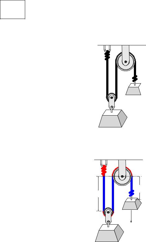
Sometimes the motion of one particle depends on the motion of another – this is called dependent motion. One situation that creates dependent motion is when two particles are connected by a cord around a pulley.

A

B

If weight A is pulled downward, weight B will be raised, but the total length of the cord, Ltotal, (assumed inextensible) is constant. The total length of the cord can be described in terms of cord lengths that

change, sA and sB, and unchanging lengths, combined and called Lconst (shown in red in the next figure.)

DATUM

sA

sB

A

0.3 m/s

B

2 sB + sA + Lconst = Ltotal

Differentiating this equation with respect to time yields the time rates of change of position, or velocities of each weight.

2 dsdtB + dsdtA + 0 = 0

2 vB = −vA

So, if weight A moves down at 0.3 m/s, weight B will move up at 0.15 m/s.

Example: Four Pulley System

At what rate, and in which direction must weight A move if weight B is to fall at a rate of 0.3 m/s?

0.3 m/s

B

A

Solution

There is a single cord between weights A and B, so the motion of one of the weights is dependent upon one the other. While the physical system is somewhat more complex than the original, 2-pulley example, the solution is not very different. The total length of the cord is made up of 9 segments, as shown in the figure below. There are 4 equivalent-length sections that lengthen as weight B is lowered. The length of each of these sections is labeled SB.

sA

B A

DATUM

sB

0.3 m/s

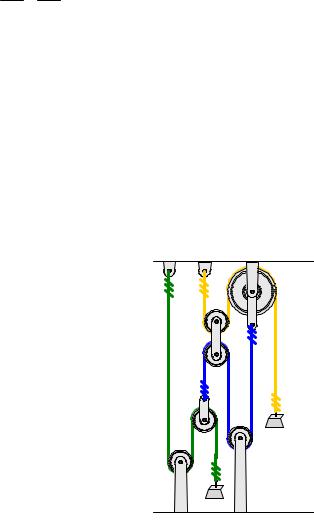
The length of the cord segment connected to weight A is labeled SA. There are four cord segments around the four pulleys that do not change as the weights move. These segments are shown in red in the figure, and their lengths are combined and called Lconst. The total cord length, then, is

4 sB + sA + Lconst = Ltotal

Differentiating this equation with respect to time yields the time rates of change of position, or velocities of each weight.

4 dsdtB + dsdtA + 0 = 0

4 vB = −vA

So, if weight B moves down at 0.3 m/s, weight A will move up at 1.2 m/s.

So far, these problems require only simple calculus, and there is little need for Mathcad’s calculational abilities. However, when there are several cords involved, Mathcad’s matrix math capabilities can come into play.

Example: Three Cord System

In the example shown below, three cords are connected around a complicated pulley system. The length of each of the cords is constant, so the sum of the segment lengths can be written for each cord.

B 0.3 m/s

A

To simplify things a bit, we first determine which segments are of constant length, shown in gray in the following figure. Then the segments that are changing length are labeled (S1 through S6, as shown in the figure.)

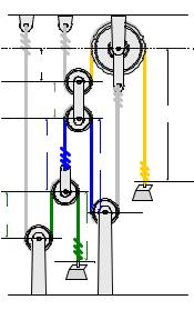
DATUM

S5

LLINK

S6

S3

S4

B 0.3 m/s

S1

S2

A

The following relationships involving the changing segment lengths can be written:

1)Segments S1 and S2, plus a fixed length, FG, sum to the total length of the green cord. LG.

2)Segments S3 and S4, plus a fixed length, FB, sum to the total length of the blue cord. LB.

3)Segments S5 and S6, plus a fixed length, FY, sum to the total length of the yellow cord. LY. Two additional relationships can be written:

4)Segments S1, S3, S5 and the length of the floating link, LLINK, sum to an unknown, but constant (fixed) length, F1.

5)Segments S4, S5 and the length of the floating link, LLINK, sum to an unknown, but constant (fixed) length, F2.

In summary, the following five equations are written:

S1 + S2 + FG = LG

S3 + S4 + FB = LB

S5 + S6 + FY = LY

S1 + S3 + S5 + LLINK = F1

S4 + S5 + LLINK = F2

Taking time derivatives, the segment lengths become velocities, and the constant terms go to zero.

v1 + v2 + 0 = 0 v3 + v4 + 0 = 0 v5 + v6 + 0 = 0

v1 + v3 + v5 + 0 = 0 v4 + v5 + 0 = 0

Since v6 is known to be 0.3 m/s (downward), these 5 equations in 5 unknowns can be solved. Including the known value, the equations become…

v1 + v2 = 0

v3 + v4 = 0

v5 = −0.3

v1 + v3 + v5 = 0 v4 + v5 = 0

To solve these simultaneous linear equations using matrix methods in Mathcad, we rewrite the equations as a coefficient matrix, C, and a right-hand-side vector, r.

	1		1	0	0	0		0
		0	0	1	1	0		0
											m
	C := 0		0	0	0	1	r :=	−0.3
											s
		1 0 1 0 1						0
						1
	0		0	0	1			0

We then invert the coefficient matrix, and multiply the inverted coefficient matrix and the r vector to obtain the unknown velocities.

	Cinv := C− 1							v := Cinv r
	0		−1	−2	1	1		0.6
		1	1	2	−1	−1
								−0.6		m
	Cinv = 0		1	1	0	−1		v = −0.3
										s
		0	0	−1	0	1		0.3
			0	1	0	0
	0							−0.3

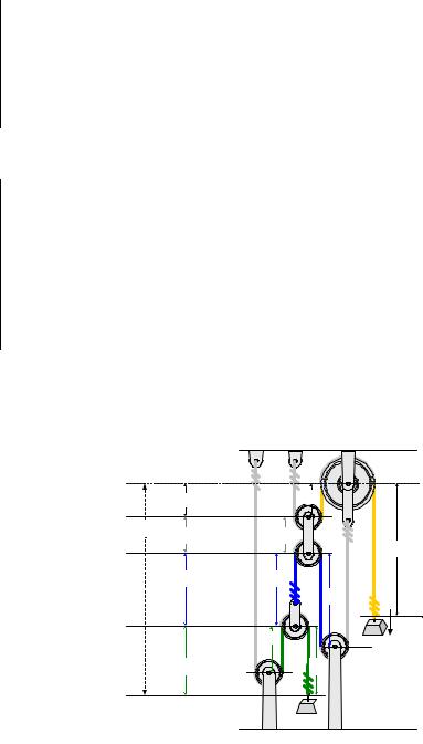
These velocities represent the rate at which segment lengths S1 through S5 are changing with time, and are not (generally) velocities relative to the datum. In order to determine the velocity of point A relative to the datum, the distance of point A relative to the datum (called LA in the figure below) must be written in terms of segment lengths.

			DATUM
	S5	S5
LA	LLINK	LLINK
			S6
	S3	S3
		S4
		B	0.3 m/s
		S1
	S2	S2

A

LA = S5 + LLINK + S3 + S2

The velocity of point A relative to the datum is the time derivative of LA.

	vA =	dLA
		dt
	=	dS5		+ 0		+	dS3	+	dS2
		dt					dt		dt

= v5 + 0 + v3 + v2

Velocities v2, v3, and v5 are known, so vA can be determined. (Note: The vector index ORIGIN in Mathcad was set to 1 for this problem.)

vA := v5 + 0 + v3 + v2 vA = −1.2 ms

Since the velocity at point B was 0.3 m/s downward, this result indicates that point A is moving at 1.2 m/s upward.

Annotated Mathcad Worksheet

Note: ORIGIN = 1 has been set using Math/Options for this problem.

Declare the coefficient matrix and right-hand-side vector

	1		1	0	0	0			0
		0	0	1	1	0			0
												m
	C := 0		0	0	0	1		r :=	−0.3
												s
		1	0	1	0	1			0
			0	0	1	1			0
	0

Invert the coefficient matrix.

			0		−1		−2	1	1
				1	1		2	−1	−1
	:= C− 1
C		C = 0 1				1		0	−1
inv		inv		0	0		−1	0	1
					0		1	0	0
			0

Multiply the inverted coefficient matrix and the right-hand-side vector to calculate the segment velocities.

		0.6
			−0.6
					m
	v := C r	v = −0.3
	inv		0.3	s
		−0.3

Use the segment velocities to calculate the velocity of point A relative to the datum.

vA := v5 + 0 + v3 + v2 vA = −1.2 ms