442 |||| CHAPTER 6 APPLICATIONS OF INTEGRATION

leaks at a constant rate and finishes draining just as the bucket reaches the 12 m level. How much work is done?

18.A 10-ft chain weighs 25 lb and hangs from a ceiling. Find the work done in lifting the lower end of the chain to the ceiling so that it’s level with the upper end.

19.An aquarium 2 m long, 1 m wide, and 1 m deep is full of water. Find the work needed to pump half of the water out

of the aquarium. (Use the fact that the density of water is 1000 kg m3.)

20.A circular swimming pool has a diameter of 24 ft, the sides are 5 ft high, and the depth of the water is 4 ft. How much

work is required to pump all of the water out over the side? (Use the fact that water weighs 62.5 lb ft3.)

21–24 A tank is full of water. Find the work required to pump the water out of the spout. In Exercises 23 and 24 use the fact that water weighs 62.5 lb ft3.

21.	3 m	22.	1 m
2 m
3 m			3 m
	8 m
23.	6 ft	24.
			12 ft
	8 ft		6 ft
	3 ft		10 ft
	frustum of a cone

;25. Suppose that for the tank in Exercise 21 the pump breaks down after 4.7 105 J of work has been done. What is the depth of the water remaining in the tank?

26.Solve Exercise 22 if the tank is half full of oil that has a density of 900 kg m3.

27.When gas expands in a cylinder with radius r, the pressure at

any given time is a function of the volume: P P V . The force exerted by the gas on the piston (see the figure) is the product of the pressure and the area: F r2P. Show that the work done by the gas when the volume expands from volume V1 to volume V2 is

W yV2 P dV

V1

x

piston head

28.In a steam engine the pressure P and volume V of steam satisfy the equation PV1.4 k, where k is a constant. (This is true for adiabatic expansion, that is, expansion in which there is no heat transfer between the cylinder and its surroundings.) Use Exer-

cise 27 to calculate the work done by the engine during a cycle when the steam starts at a pressure of 160 lb in2 and a volume of 100 in3 and expands to a volume of 800 in3.

29.Newton’s Law of Gravitation states that two bodies with masses m1 and m2 attract each other with a force

F G m1m2 r2

where r is the distance between the bodies and G is the gravitational constant. If one of the bodies is fixed, find the work needed to move the other from r a to r b.

30.Use Newton’s Law of Gravitation to compute the work required to launch a 1000-kg satellite vertically to an orbit 1000 km high. You may assume that the earth’s mass is 5.98 1024 kg and is concentrated at its center. Take the

radius of the earth to be 6.37 106 m and G 6.67 10 11 N m2 kg2.

				6.5
T
15
10
5
	6			Tave
0	12	18	24	t

FIGURE 1

AVERAGE VALUE OF A FUNCTION

It is easy to calculate the average value of finitely many numbers y1, y2, . . . , yn:

yave y1 y2 yn n

But how do we compute the average temperature during a day if infinitely many temperature readings are possible? Figure 1 shows the graph of a temperature function T t , where t is measured in hours and T in C, and a guess at the average temperature, Tave.

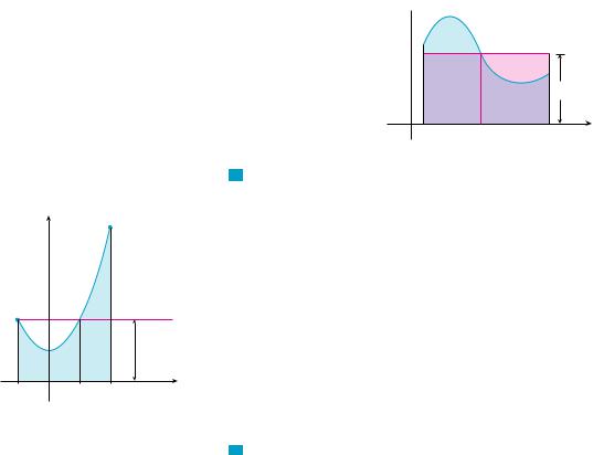
In general, let’s try to compute the average value of a function y f x , a x b. We start by dividing the interval a, b into n equal subintervals, each with lengthx b a n. Then we choose points x*1 , . . . , x*n in successive subintervals and cal-

N For a positive function, we can think of this definition as saying

area average height width

SECTION 6.5 AVERAGE VALUE OF A FUNCTION |||| 443

culate the average of the numbers f x*1 , . . . , f x*n :

f x1* f x*n

n

(For example, if f represents a temperature function and n 24, this means that we take temperature readings every hour and then average them.) Since x b a n, we can write n b a x and the average value becomes

f x1* f xn*				1	f x1* x f xn* x
	b a			b a
	x
				1	n
					f xi* x
				b a
					i 1

If we let n increase, we would be computing the average value of a large number of closely spaced values. (For example, we would be averaging temperature readings taken every minute or even every second.) The limiting value is

		1	n	1
	lim		f x*i x		b f x dx
				b a
	n l b a i 1				ya

by the definition of a definite integral.

Therefore we define the average value of f on the interval a, b as

1		b
fave		ya f x dx
	b a

V EXAMPLE 1 Find the average value of the function f x 1 x2 on the interval 1, 2 .

SOLUTION With a 1 and b 2 we have

1			1				1		x3	2
		b		2				x		1
fave		ya f x dx		y 1	1	x2 dx					2 M
	b a		2 1				3		3

If T t is the temperature at time t, we might wonder if there is a specific time when the temperature is the same as the average temperature. For the temperature function graphed in Figure 1, we see that there are two such times––just before noon and just before midnight. In general, is there a number c at which the value of a function f is exactly equal to the average value of the function, that is, f c fave? The following theorem says that this is true for continuous functions.

THE MEAN VALUE THEOREM FOR INTEGRALS If f is continuous on a, b , then there exists a number c in a, b such that

		1		b
	f c	fave		ya f x dx
			b a
that is,	yb f x dx f c b a

a

444 |||| CHAPTER 6 APPLICATIONS OF INTEGRATION

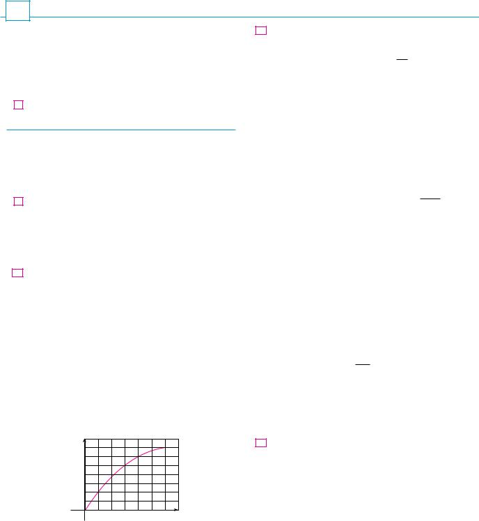
N You can always chop off the top of a (twodimensional) mountain at a certain height and use it to fill in the valleys so that the mountaintop becomes completely flat.

The Mean Value Theorem for Integrals is a consequence of the Mean Value Theorem for derivatives and the Fundamental Theorem of Calculus. The proof is outlined in Exercise 23.

The geometric interpretation of the Mean Value Theorem for Integrals is that, for positive functions f, there is a number c such that the rectangle with base a, b and height f c has the same area as the region under the graph of f from a to b. (See Figure 2 and the more picturesque interpretation in the margin note.)

y

y=ƒ

f(c)=fave

FIGURE 2	0	a	c	b	x

	y			(2,5)
		y=1+≈
(_1,2)
				fave=2
_1	0	1	2	x

FIGURE 3

V EXAMPLE 2 Since f x 1 x2 is continuous on the interval 1, 2 , the Mean Value Theorem for Integrals says there is a number c in 1, 2 such that

y21 1 x2 dx f c 2 1

In this particular case we can find c explicitly. From Example 1 we know that fave 2, so the value of c satisfies

	f c fave 2
Therefore	1 c2 2 so c2 1

So in this case there happen to be two numbers c 1 in the interval 1, 2 that work in the Mean Value Theorem for Integrals. M

Examples 1 and 2 are illustrated by Figure 3.

V EXAMPLE 3 Show that the average velocity of a car over a time interval t1, t2 is the same as the average of its velocities during the trip.

SOLUTION If s t is the displacement of the car at time t, then, by definition, the average velocity of the car over the interval is

s		s t2 s t1
t		t2 t1

On the other hand, the average value of the velocity function on the interval is

		1	t2				1	t2
vave			yt1	v t dt				yt1	s t dt
	t2	t1				t2 t1
		1	s t2 s t1				(by the Net Change Theorem)
	t2	t1
	s t2 s t1				average velocity					M
		t2 t1

6.5EXERCISES

1– 8 Find the average value of the function on the given interval.

1.	f x 4x x 2, 0, 4					2.	f x sin 4 x, ,
							2
3.	3			1, 8		4.		s1		x 3 ,		0, 2
	t x sx ,						t x x
5.	f t te t 2, 0, 5
6.	f sec2 2 ,				0, 2
7.	h x cos4x sin x,				0,

8. h u 3 2u 1, 1, 1

9–12

(a)Find the average value of f on the given interval.

(b)Find c such that fave f c .

(c)Sketch the graph of f and a rectangle whose area is the same as the area under the graph of f.

9.		f x x 3 2, 2, 5
10.		f x s		, 0, 4
			x
; 11.		f x 2 sin x sin 2x, 0,
;12.		f x 2x 1 x 2 2, 0, 2

13.If f is continuous and x13 f x dx 8, show that f takes on the value 4 at least once on the interval 1, 3 .

14.Find the numbers b such that the average value of

f x 2 6x 3x 2 on the interval 0, b is equal to 3.

15. The table gives values of a continuous function. Use the Midpoint Rule to estimate the average value of f on 20, 50 .

x	20	25	30	35	40	45	50
f x	42	38	31	29	35	48	60

16. The velocity graph of an accelerating car is shown.

(a) Estimate the average velocity of the car during the first 12 seconds.

(b) At what time was the instantaneous velocity equal to the average velocity?

√
(km/h)
60
40
20
0	4	8	12	t (seconds)

SECTION 6.5 AVERAGE VALUE OF A FUNCTION |||| 445

17.In a certain city the temperature (in F) t hours after 9 AM was modeled by the function

t

T t 50 14 sin

12

Find the average temperature during the period from 9 AM to 9 PM.

18.(a) A cup of coffee has temperature 95 C and takes 30 minutes to cool to 61 C in a room with temperature 20 C. Use Newton’s Law of Cooling (Section 3.8) to show that the temperature of the coffee after t minutes is

T t 20 75e kt

where k 0.02.

(b)What is the average temperature of the coffee during the first half hour?

19.The linear density in a rod 8 m long is 12 sx 1 kg m, where x is measured in meters from one end of the rod. Find the average density of the rod.

20.If a freely falling body starts from rest, then its displacement is given by s 12 tt 2. Let the velocity after a time T be vT . Show that if we compute the average of the velocities with

respect to t we get vave 12 vT , but if we compute the average of the velocities with respect to s we get vave 23 vT.

21.Use the result of Exercise 79 in Section 5.5 to compute the average volume of inhaled air in the lungs in one respiratory cycle.

22.The velocity v of blood that flows in a blood vessel with radius R and length l at a distance r from the central axis is

v r P R2 r 2

4 l

where P is the pressure difference between the ends of the vessel and is the viscosity of the blood (see Example 7 in Section 3.7). Find the average velocity (with respect to r) over the interval 0 r R. Compare the average velocity with the maximum velocity.

23.Prove the Mean Value Theorem for Integrals by applying the

Mean Value Theorem for derivatives (see Section 4.2) to the function F x xax f t dt.

24. If fave a, b denotes the average value of f on the intervala, b and a c b, show that

	fave a, b	c a	fave a, c	b c	fave c, b
		b a		b a