suai.ru/our-contacts

quantum machine learning

J.B. Broekaert, et al.

Cognitive Psychology 117 (2020) 101262

gender was .489. A non-significant gender bias was present in the random assignment of participants in the U-to-K vs K-to-U flows.4 We point out that in our experiment no actual rewards were being given nor were true monetary risks being taken by the participants. Only a flat fee for participation to the task was given to each participant. There is no evidence that true monetary rewards would produce less random performance in this paradigm. The pioneering study of Tversky and Shafir (1992), which showed a strong DE, did not involve real monetary risks, and the same applies to most subsequent replications. An exception is the work of Kühberger et al. (2001) who used real monetary risks in one of their conditions. Specifically, their procedure involved tricking students into risking their proper money first and then surprise remitting their debts at the end. 5 At face value, such a procedure should encourage more attentive behavior. However, Kühberger et al. (2001) did not find any differences in behavior between the condition with real monetary risks and a condition with gambles on hypothetical money. Such a powerful null result casts doubt on the effectiveness of (small) monetary risks and rewards in affecting participants’ behavior in the two-stage gamble paradigm. This conclusion is consistent with the general impression that small monetary incentivization is not effective in biasing behavior. For example, Camerer and Hogarth (1999) concluded that “there is no replicated study in which a theory of rational choice was rejected

at low stakes in favor of a well-specified behavioral alternative and accepted at high stakes” (p.23).

3. Experimental results.

3.1. Experiment 1

The within-participants segment of Experiment 1 showed no indication for a Disjunction Effect at any of the payoff values of X (see Fig. S5 in SM 9). We recall that contrary to the approach of Tversky and Shafir (1992) we distinguish between the violation of the LTP and the violation of the STP, Section 1.1. The aggregate probability to take the second-stage gamble in the Unknown previous outcome condition consistently satisfied the LTP over the payoff range. Also the gamble pattern distributions showed no indication for STP violation, which should have been apparent through the statistical dominance of gamble pattern (g|W , g|L, s|U) (the distribution data corresponding to X = 2 are included in Table 2).

In the between-participants segment of Experiment 1 we found a marginally significant inflative violation of LTP for lower values of the payoff variable X, most clearly at X = .5 with p (g|W ) = 0.68, p (g|L) = 0.71 and p (g|U) = 0.87. Based on contingency counts a left-tailed Fisher test for increased association of Gamble/Stop by Win/Unknown at pay-off at X = .5 showed a significance of p = .0176, with odds ratio 0.45 and CI = [0.22, 0.91] for = .05. Applying the Holm-Bonferroni correction for the five measurements over the payoff range renders the inflative effect of p (g|U) at X=.5 non-significant (uncorrected p-values over the X-range:

{.02, .22, .85, .96, .92}).

Finally we remark that in both the within-participants and the between-participants design the participants clearly distinguished the Lose outcome and Win outcome condition such that a larger preference was given to taking the gamble under Lose outcome condition than under Win outcome –an observation which runs counter to reported data on the two-stage gamble experiment (Tversky & Shafir, 1992; Kühberger et al., 2001; Lambdin & Burdsal, 2007; Surov, Pilkevich, Alodjants, & Khmelevsky, 2019).

3.2. Experiment 2

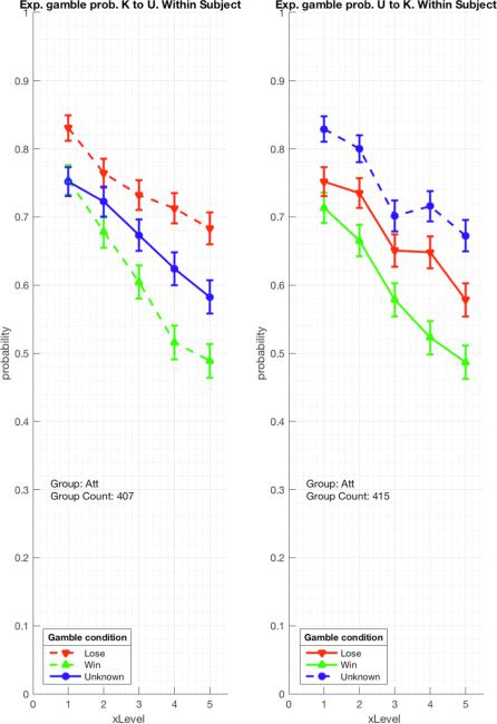
The full participant group was subdivided by condition flow order in Experiment 2. This allows an observation of a major effect on choice probability due to the block ordering, Fig. 3. In the flow order when the Unknown conditioned block precedes the Known conditioned block the LTP is violated over the whole X-range in an inflative manner p = 6.25e 06, (N = 415), by Wilcoxon signed rank test. The Wilcoxon signed-rank test was used to assess the paired differences –Lose conditioned outcome response versus Unknown conditioned outcome response– from repeated measurements on a single sample. The test allows to compare the effect of two conditions on paired outcomes –here in particular to test whether the participants gamble more on Unknown vs Known outcome conditions. It is a non-parametric test which does not assume a normally distributed population (the data range from 0 to 1 in fractions 1/5), nor does it require equal variance, and independence of the errors. For each participant the X-averaged score under Lose and Unknown outcome conditions was compared and tested for H0 hypothesis that p(g|U, X ) X < p (g|L, X ) X .

On the contrary, in the flow order where the Known block precedes the Unknown block the LTP is satisfied over the whole X-range (N = 407), Fig. 3. The decreasing tendency to gamble under increasing payoff and the differing reaction of participants to secondstage gambles conditioned on W or L are observed in both gamble order conditions.

The design and sample size of Experiment 2 allowed us to analyse the gamble probabilities for different categories of participants. In the first instance we looked at the observed gamble probabilities for the full group by flow order, in the next sections we partition those two flow ordered groups by risk attitude –more vs less risk averse. 6

4 Based on contingency counts a Fisher test for non-random association between flow order and gender showed p = .13 (two-tailed), with odds ratio 0.81 and confidence interval CI = [0.61, 1.06] for = .05.

5Note, such a procedure may introduce a sampling bias, since the participants who decide to take part in such a study would be expected to be more risk seeking.

6A further partitioning by gamble pattern range, based on ID-score, eq. (S3), is provided in the Supplementary Materials, SM 4.

8

suai.ru/our-contacts

quantum machine learning

J.B. Broekaert, et al.

Cognitive Psychology 117 (2020) 101262

Fig. 3. Experimental gamble probabilities, on the left for participants in K-to-U order, on the right for U-to-K order. In the U-to-K order an inflative Disjunction Effect occurs. The payoff parametrised by XLevel [1, 5] appears on the x-axis. Error bars represent the standard error of the mean.

3.2.1. More versus less risk averse participants

Considering that it is behavior relative to gambles that is at stake, it seems a shortcoming in both the original Tversky and Shafir (1992) work and later extensions that the risk aversion of participants has not been taken into account. In order to operationally characterise the risk aversion of participants their choices in the single-stage gambles were used. We recall the single-stage gambles are the same as the condition-free first stage of the two-stage gamble. By experimental design in Experiment 2 each participant is twice presented with all the single-stage gambles, once in the Known block and once in the Unknown block. We use the sum total of the instances a participant accepts the initial gamble as the operational measure of risk attitude. In our design this ‘single-gamble score’ can vary from 0 to 10. A high single-gamble score indicates a participant who frequently chooses to gamble, despite the potential loss, hence expressing low risk aversion. A low single-gamble score indicates a participant with higher risk aversion since these participants do refrain more often from a risky choice with potential loss.

9

suai.ru/our-contacts

quantum machine learning

J.B. Broekaert, et al. Cognitive Psychology 117 (2020) 101262

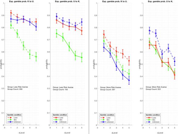
From Fig. S3, we observe that a substantial fraction of the participants obtained a single-gamble score of 10. Participants that always take the initial gamble, regardless the payoff, can be considered more risk-seeking than participants that will not always take it. This criterion warrants a partitioning of the sample by either obtaining a single-gamble score less than 10 or the maximum of 10, resulting in a ‘More risk averse’ group (N = 429) and a ‘Less risk averse’ group (N = 393) which are approximately of the same size.7 A first overall observation of the second-stage gamble probabilities separated along our criterion for risk attitude, Fig. 4 confirms some basic expectations. The defined ‘More risk averse’ group is indeed more risk averse than the defined ‘Less risk averse’ group, since all gamble probabilities for all payoff values X and for all outcome conditions are lower in the ‘More risk averse’ group in comparison to the same gambles taken by the ‘Less risk averse’ group. Moreover, the ‘More risk averse’ participants have a faster diminishing motivation to take the second-stage gamble for increasing payoff X when the first-stage gamble outcome was Lose or Unknown. However, when the first-stage gamble outcome was Win, this diminishing motivation to gamble over X remains the same for both groups. The ‘Less risk averse’ participants also show a significant distinction between gamble choices under W and L condition, while the ‘More risk averse’ participants hardly discriminate between these two conditions.8

A major and rather surprising observation for the ‘More risk averse’ group is the strong flow-order with outcome-condition crossover interaction (Fig. 4, right panel). Remarkably the ‘More risk averse’ participants show a tendency for a Disjunction Effect in K-to- U order and a significant inflative violation of the LTP in U-to-K order. Notice that this is a between-participants effect of flow order. A mixed ANOVA with unbalanced design (N = 207/N = 222) and with a dependent variable gamble probabilities (averaged across all payoffs X) and independent variables first-stage gamble outcome condition {W, L, U} and order {‘K-to-U’, ‘U-to-K’} revealed a significant interaction, F (2, 1281) = 12.78, p = 3. 20e 06 .

By contrast, there were no main effects for either first-gamble outcome condition or order in the ‘More risk averse’ group. That is, surprisingly, there appears to be no effect on choice behavior from whether the first-stage gamble was indicated as Won or Lost.

The ‘Less risk averse’ participants do not show any tendency for a Disjunction Effect in the order K-to-U, while in the U-to-K order a non-significant tendency for an inflative violation of the LTP occurs. A mixed ANOVA with unbalanced design (N = 200/N = 193), testing for factors of condition {W, L, U} and order {‘K-to-U’, ‘U-to-K’}, revealed a significant main effect of condition {W, L, U} F (2, 1173) = 43.88, p = 4. 2e 19 . Therefore, in this group a substantial difference in gambling probability is observed, depending on whether the first-stage gamble was Won or Lost.

In the U-to-K order the ‘More risk averse’ participants are mostly indifferent to choice under the Win or Lose first-stage gamble outcome condition, therefore the inflative violation of the LTP has to be tested with respect to both choices of the two Known outcome conditions. To test the statistical significance of the violation of the LTP the Wilcoxon test for repeated measurements on a single sample was applied. The test was used to assess the paired difference from measurements on Known and Unknown conditions for each participant. The Wilcoxon test shows a significant violation of the LTP, with p = 1.7e-06 (N = 222) for H0 that

p(g|U, X ) X < p (g|L, X ) X and p = .0002 (N = 222), for H0 that p(g|U, X ) X < p (g|W , X ) X .

In the K-to-U order the ‘More risk averse’ participants show a small but consistent diminished choice probability under Win in comparison to the Lose first-stage gamble outcome condition. In this case therefore the Disjunction Effect is tested between the choices in the Unknown and Win outcome conditions only. The Wilcoxon test shows a significant Disjunction Effect, with p = .045

(N = 207), for H0 that p(g|U, X ) X > p (g|W , X ) X . Since this result seems marginally significant, we also applied the Pratt correction to the Wilcoxon test (by modification of Matlab code in Cardillo (2006)). The Pratt correction is required for samples with frequent ties, which typically occur in discrete distributions like in our present data set where the compared X-averaged gamble response values are fractions ranging from 0/5 till 5/5. While the Wilcoxon test eliminates all zero differences of measurement outcomes, the Pratt correction keeps the zero differences in the ranking procedure of the statistical test (Pratt, 1959). Using the Pratt correction, the Disjunction Effect for ‘More risk averse’ participants in the K-to-U order is marginally not statistically significant anymore at p = .062 (N = 207).

The size of the sample allows insight in decision patterns besides aggregate gamble probability. In particular we can consider the prevalence of particular gamble strategies expressed as WLU gamble patterns, Fig. 5. Three gamble patterns have a deflative effect on the average gamble probability under Unknown condition –(g|W , s|L, s|U), (s|W, g|L, s|U ) and (g|W , g|L, s|U)– and three have an inflative effect – (g|W , s|L, g|U), (s|W, g|L, g|U) and (s|W , s|L, g|U), Table S1. The probability distribution over the patterns causes the occurrence of either a Disjunction Effect or an inflative violation of the Law of Total Probability. It is therefore important to analyse the distribution of the gamble patterns over the spectrum of payoff parameter X, Fig. 5.

A remarkable difference between the pattern distribution of the ‘Less risk averse’ and ‘More risk averse’ participants occurs over the range of increasing payoff X. In ‘Less risk averse’ participants the modal strategy remains ‘always play’, (g|W , g|L, g|U ), throughout the X range. In the ‘More risk averse’ participants the modal pattern changes from ‘always play’ at the lowest payoff to ‘never play’, or (s|W , s|L, s|U), at the highest payoff.

7 The demographics for the ‘Less risk averse’ group with respectively NKU = 200 and NUK = 193 participants revealed respective gender means

mgender = 0.61 and mgender = 0.52, while the ‘More risk averse’ group had NKU = 207 and NUK = 222 participants, with respective gender means

mgender = 0.48 and mgender = 0.46. Therefore a small gender bias was present due to our risk-aversion partitioning, (p = .006, two-tailed) where the
odds ratio is 0.68 and the confidence interval CI = [0.52, 0.89] for		=	.05	.
8
	In SM 10, we analyse the effect of informing the participant about the Unknown outcome of the first-stage in a two-stage gamble by comparing

the probability of taking the single-stage gamble p(g) (thus without any condition set by an earlier stage gamble) and the second-stage gamble p(g|U ) (in which the participant is informed that the outcome is Unknown). This analysis is done for ‘more risk averse’ participants, since for ‘less risk averse’ participants p(g) = 1 for all X, hence further analysis is not pertinent for the latter participant group.

10

suai.ru/our-contacts

quantum machine learning

J.B. Broekaert, et al.

Cognitive Psychology 117 (2020) 101262

Fig. 4. Observed gamble probabilities for sample partitions into ‘Less risk averse’ (left panel), and ‘More risk averse’ (right panel). Within each panel, on the left are the observations for the K-to-U order, on the right the U-to-K order. The ‘More risk averse’ participants show a significant inflative violation of the Law of Total Probability in U-to-K order, and a marginally significant Disjunction Effect, or deflative violation of the Law of

Total Probability, in K-to-U order. The payoff parametrised by XLevel [1, 5] appears on the x-axis. Error bars represent the standard error of the mean.

The pattern (s|W , g|L, g|U) (‘only stop on Win’ strategy) is the second most common pattern over the X range for ‘Less risk averse’ participants. In the ‘More risk averse’ participants, the patterns with ‘stop on U’ strategy become more frequent only for higher values of X (reflected in the decreasing of p (g|U, X ) with increasing X). In general we observe that ‘More risk averse’ participants resort to a larger variety of gamble patterns when X increases. In the ‘Less risk averse’ group the near inflative p (g|U, X ) originates mainly from the probability mass in the pattern (s|W , g|L, g|U), in both flow orders.

In sum, in the ‘More risk averse’ group the marginally significant DE in the K-to-U order emerges due to the empirical preponderance of all patterns with deflative effect over patterns with inflative effect, while in the U-to-K order the inflative violation of the LTP emerges through the preponderance of all patterns with inflative effect over the deflative patterns. The Disjunction Effect and the inflative violation of the Law of Total Probability are therefore not caused by their purported association to (g|W , g|L, s|U) or (s|W , s|L, g|U) patterns. This still leaves open the question of whether some individual participants might adhere to specific deflative or inflative strategies over the X-range of payoffs, and whether these tendencies are masked by the aggregation of data (Estes, 1956). This issues is addressed in Supplementary Materials Section SM 3.

To end this section we discuss the concern that these participants whom we labeled ‘less risk averse’ would simply ‘click through’ the experiment rather than informedly choose to always play a single-stage gamble. To avoid the possibility that this type of ‘lazy responding’ effect could take place, in our survey code in Qualtrics we implemented a random Display Order of the gamble button and the stop button. The gamble button could appear on either of two locations, on the left or the right of the screen. With each new gamble, it was randomly determined whether the gamble button was on the right or on the left. A lazy participant would be expected to click through at the same location, which would lead to equivalent proportions of gamble and stop decisions. By contrast, the ‘less risk averse’ participants would need to hunt the gamble button, at the different screen locations where it would appear, in order to adhere to an ‘always gamble’ strategy. This commitment is not in line with laziness for it requires attention and takes more time to perform than robotically clicking the same button appearing randomly below their cursor. In fact the average task duration for ‘Less

11

suai.ru/our-contacts

quantum machine learning

J.B. Broekaert, et al.

Cognitive Psychology 117 (2020) 101262

Fig. 5. Experimental gamble pattern probabilities in the WLU order arranged from (s|W , s|L, s|U) to (g|W , g|L, g|U ); in the left panel we show ‘Less risk averse’ participants, in the right panel ‘More risk averse’ participants. The patterns have been ordered in WLU order with 1 for ‘gamble’ and 0 for ‘stop’. The patterns for payoff parameter X = .5 is shown at the top and increasing to X = 4 at the bottom. The four ‘gamble-on-U’ patterns (XYg) are grouped to the right on the X-axis, the four ‘stop-on-U’ patterns (XYs) are grouped to the left. The probabilities for the K-to-U order appear on the left (pink color) and for U-to-K on the right (teal color). For comparison the yellow markers in the X = 2 panel indicate the pattern probabilities of Tversky and Shafir (1992). In the right panel for ‘More risk averse’ participants one observes the probability mass shifting from XYg to XYs patterns for increasing payoff, corresponding to the decreasing gamble probability p(g|U, X ) with increasing X. Error bars represent the standard error of the mean.

risk	averse’	participants is indeed somewhat longer than for ‘More risk averse’ participants,		Mduration,Lra	=	652s while
			9
Mduration,Lra = 621s.

Additionally, from the perspective of Expected Value the choices made by the ‘less risk averse’ participants make sense. This is

because all these gambles have an Expected Value which exceeds not playing the gambles by an amount of 25X (see SM 12). Therefore it makes sense to always play the single-stage and even to always play the second-stage gambles as well.10

Another relevant point is that participants defined as ‘less risk averse’ do not always play all gambles and show a decreasing tendency to take the second-stage gambles for higher pay-offs (see Fig. 4). They meaningfully (i.e., on the basis of a non-random pattern) change their choices depending on outcome condition and payoff size (less so on order).

Finally, it is worth bearing in mind that participants that always play single-stage and second-stage gambles have no influence in creating inflation nor deflation of the probability P (g|U). The (g|W , g|L, g|U ) pattern contributes equally to each gamble probability. So, the small percentage of true always takers have a perfectly neutral effect on the ordering of the probabilities (their elimination would scale up the small inflation effect in the U-to-K flow for the less risk averse participants).

9A two-sample t-test for the null hypothesis that the task duration in ‘less risk averse’ and ‘more risk averse’ players have equal means and equal but unknown variances accepts the null hypothesis; p = .4, CI = [-45.9, 107.0], t = 0.79, df = 820, sd = 558.

10A quote of the voluntary feedback of one of the ‘true’ always takers reveals this participant’s motivation: “I’m not usually a gambler but unless I misunderstood the directions, it was always monetarily wise to flip the coin again. If you win, you have a chance to win again and if you lose you only lose half the amount and have a better chance of winning on the next.” Similarly ‘never takers’ can act by consistent strategy as well, even if it is against the expected value of each gamble. It is of interest to quote the voluntary feedback of two of those ‘never players’: “I think gambling is foolish. I would never put money at risk”, and “My parents are addicted to gambling so I really don’t like to gamble myself.”

12