one-loop

2	2	2		2	2	2
+ mf	C0[m1 , m2 , 0, mf , ms , mf ]
In[15]:= Coefficient[PaVeReduce[DL],AR							BR]
			2	2	2		2	2	2
	m2 mf B0[m1 , mf , ms ]					m2 mf B0[m2 , mf , ms ]
Out[15]= -----------------------						- -----------------------
		2		2			2	2
		m1	- m2				m1 - m2
		2	2		2	2	2
+ m2 mf C0[m1 , m2 , 0, mf , ms , mf ]
(*******************				End of	Mathematica output			**********************)

From these expressions one can immediately verify that the divergences cancel in DL;R and that they are not present in CL;R. To nish this section we just rewrite the CL;R in our usual notation. We get

CL	=		e Q`	ALBLmF C0(0; m22; m12; mF2 ; mF2 ; mS2 ) C2	(0; m12; m22; mF2 ; mF2 ; mS2 )
			16 2
				+ALBRm2 C2(0; m12; m22; mF2 ; mF2 ; mS2 ) + C12(0; m12; m22; mF2 ; mF2 ; mS2 )
				+C22(0; m12; m22; mF2 ; mF2 ; mS2 )
				+ ARBLm1 C12(0; m12; m22; mF2 ; mF2 ; mS2 )	(6.15)
CR	=	CL(L $ R)			(6.16)

These equations are in agreement with Eqs. (32-34) and Eqs. (38-39) of Ref. [9], although some work has to be done in order to verify that11. This has to do with the fact that the PV decomposition functions are not independent (see the Appendix for further details on this point). We can however use the power of FeynCalc to verify this. We list below a simple program to accomplish that.

(******************** Program lavoura-ns.m **************************)

(*

This program tests the results of my program mueg-ns.m against the results obtained by L. Lavoura (hepph/0302221).

*)

(* First load FeynCalc.m and mueg-ns.m *)

11An important di erence between our conventions and those of Ref. [9] is that p1 and p2 (and obviously m1 and m2) are interchanged.

50

<<FeynCalc.m

<<mueg-ns.m

(*

Now write Lavoura integrals in the notation of FeynCalc. Be careful with the order of the entries.

*)

c1:=PaVe[1,{m2^2,0,m1^2},{ms^2,mf^2,mf^2}]

c2:=PaVe[2,{m2^2,0,m1^2},{ms^2,mf^2,mf^2}]

d1:=PaVe[1,1,{m2^2,0,m1^2},{ms^2,mf^2,mf^2}]

d2:=PaVe[2,2,{m2^2,0,m1^2},{ms^2,mf^2,mf^2}]

f:=PaVe[1,2,{m2^2,0,m1^2},{ms^2,mf^2,mf^2}]

(* Write Eqs. (32)-(34) of hepph/0302221 in our notation *)

k1:=PaVeReduce[m2*(c1+d1+f)]

k2:=PaVeReduce[m1*(c2+d2+f)]

k3:=PaVeReduce[mf*(c1+c2)]

(*

Now test the results. For this we should use the equivalences:

\rho -> AL BR \lambda -> AR BL

\xi	->	AR	BR
\nu	->	AL	BL
*)

testCLALBR:=Simplify[PaVeReduce[Coefficient[CL, AL BR]-k1]] testCLARBL:=Simplify[PaVeReduce[Coefficient[CL, AR BL]-k2]] testCLALBL:=Simplify[PaVeReduce[Coefficient[CL, AL BL]-k3]]

testCRALBR:=Simplify[PaVeReduce[Coefficient[CR, AL BR]-k2]] testCRARBL:=Simplify[PaVeReduce[Coefficient[CR, AR BL]-k1]] testCRARBR:=Simplify[PaVeReduce[Coefficient[CR, AR BR]-k3]]

(****************** End of Program lavoura-ns.m **********************)

One can easily check that the output of the six tests is zero, showing the equivalence between our results. And all this is done in a few seconds.

51

6.2Charged scalar neutral fermion loop

We consider now the case of the scalar being charged and the scalar neutral. The general case of both charged [9] can also be easily implemented, but for simplicity we do not consider it here. The couplings are now

l -

F 0

S - i ( A

L

P

L

+ A

R

P

R

)

S +i (B

L

P

L

+B

R

P )

R

F 0

l -

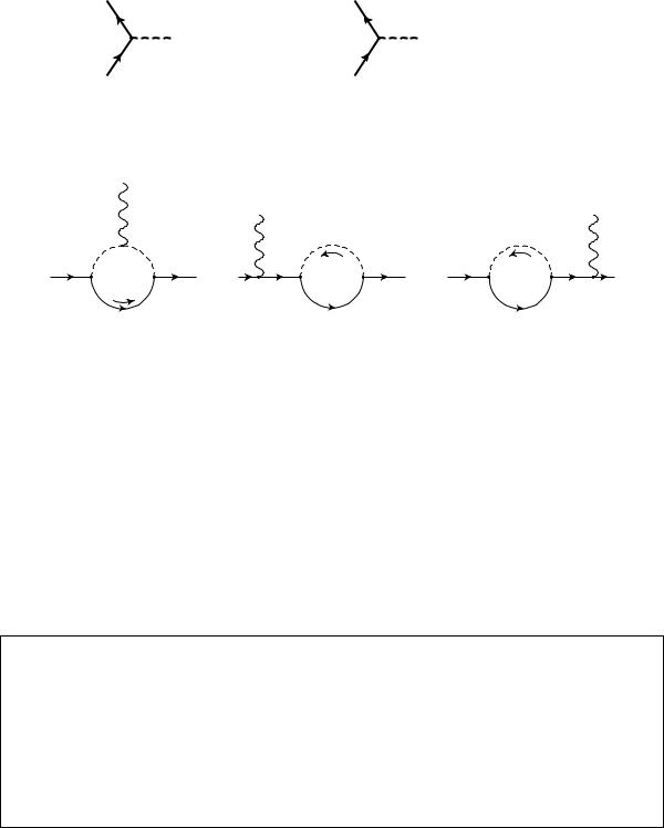
and the diagrams contributing to the process are given in Fig. 14, where all the denomi-

k
			k		D1	k
D’3	D’2		D1
			q	p1 p2		p1
p2	p1	p2			q
q			D5		D7
D’1			D4		D6
1)			2)		3)
			Figure 14:
nators are as in Eqs. (6.2)- (6.4) except that
D10 = q2 mF2	; D20	= (q p1)2 mS2 ;		D30 = (q p1 k)2 mS2		(6.17)
Also the coupling of the photon to the charged scalar is, in our notation,
		ie Q` ( 2q + p1 + p2)				(6.18)

The procedure is very similar to the neutral scalar case and we just present here the mathematica program and the nal result. All the checks of niteness and gauge invariance can be done as before.

(************************ Program mueg-cs.m ***************************)

(*

This program calculates the COMPLETE (both the 3 point amplitude and the two self energy type on each external line) amplitudes for

\mu -> e \gamma when the fermion line in the loop is neutral and the charged line is a scalar. The \mu has momentum p2 and mass m2, the electron (p1,m1) and the photon momentum k. The momentum in the loop is q.

52

The assumed vertices are,

1) Electron-Scalar-Fermion:

Spinor[p1,m1] (AL P_L + AR P_R) Spinor [pf,mf]

2) Fermion-Scalar-Muon:

Spinor[pf,mf] (BL P_L + BR P_R) Spinor [p2,m2]

*)

dm[mu_]:=DiracMatrix[mu,Dimension->4] dm[5]:=DiracMatrix[5] ds[p_]:=DiracSlash[p] mt[mu_,nu_]:=MetricTensor[mu,nu] fv[p_,mu_]:=FourVector[p,mu] epsilon[a_,b_,c_,d_]:=LeviCivita[a,b,c,d] id[n_]:=IdentityMatrix[n] sp[p_,q_]:=ScalarProduct[p,q] li[mu_]:=LorentzIndex[mu]

L:=dm[7]

R:=dm[6]

(* SetOptions[{B0,B1,B00,B11},BReduce->True] *)

gA:= AL DiracMatrix[7] + AR DiracMatrix[6]

gB:= BL DiracMatrix[7] + BR DiracMatrix[6]

num1:= Spinor[p1,m1] . gA . (ds[q]+mf) . gB . Spinor[p2,m2] \ PolarizationVector[k,mu] ( - 2 fv[q,mu] + fv[p1,mu] + fv[p2,mu] )

num11:=DiracSimplify[num1];

num2:=Spinor[p1,m1] . gA . (ds[q]+ds[p1]+mf) . gB . (ds[p1]+m2) . \ ds[Polarization[k]] . Spinor[p2,m2]

num3:=Spinor[p1,m1] . ds[Polarization[k]] . (ds[p2]+m1) . gA . \ (ds[q]+ds[p2]+mf) . gB . Spinor[p2,m2]

SetOptions[OneLoop,Dimension->D]

53

amp1:=num1 \ FeynAmpDenominator[PropagatorDenominator[q,mf],\

PropagatorDenominator[q-p1,ms],\

PropagatorDenominator[q-p1-k,ms]]

amp2:=num2 \ FeynAmpDenominator[PropagatorDenominator[q+p1,mf], \

PropagatorDenominator[p2-k,m2], \ PropagatorDenominator[q,ms]]

amp3:=num3 \ FeynAmpDenominator[PropagatorDenominator[p1+k,m1], \

PropagatorDenominator[q+p2,mf], \ PropagatorDenominator[q,ms]]

(* Define the on-shell kinematics *)

onshell={ScalarProduct[p1,p1]->m1^2,ScalarProduct[p2,p2]->m2^2, \ ScalarProduct[k,k]->0,ScalarProduct[p1,k]->(m2^2-m1^2)/2, \ ScalarProduct[p2,k]->(m2^2-m1^2)/2, \ ScalarProduct[p2,Polarization[k]]->p2epk, \ ScalarProduct[p1,Polarization[k]]->p2epk}

(* Define the divergent part of the relevant PV functions*)

div={B0[m1^2,mf^2,ms^2]->Div,B0[m2^2,mf^2,ms^2]->Div, \ B0[0,mf^2,ms^2]->Div,B0[0,mf^2,mf^2]->Div,B0[0,ms^2,ms^2]->Div}

res1:=(-I / Pi^2) OneLoop[q,amp1] res2:=(-I / Pi^2) OneLoop[q,amp2] res3:=(-I / Pi^2) OneLoop[q,amp3]

res:=res1+res2+res3 /. onshell

auxT1:= res1 /.onshell auxT2:= PaVeReduce[auxT1] auxT3:= auxT2 /. div

divT:=Simplify[Div*Coefficient[auxT3,Div]]

auxS1:= res2 + res3 /.onshell auxS2:= PaVeReduce[auxS1] auxS3:= auxS2 /. div

divS:=Simplify[Div*Coefficient[auxS3,Div]]

54

(* Check cancellation of divergences

testdiv should be zero because divT=-divS

*)

testdiv:=Simplify[divT + divS]

(* Extract the different Matrix Elements

Mathematica writes the result in terms of 6 Standard Matrix Elements. To have a simpler result we substitute these elements by simpler expressions (ME[1],...ME[6]). Not all are independent.

{StandardMatrixElement[p2epk u[p1, m1] . ga[6] . u[p2, m2]],

StandardMatrixElement[p2epk u[p1, m1] . ga[7] . u[p2, m2]],

StandardMatrixElement[p2epk u[p1, m1] . gs[k] . ga[6] . u[p2, m2]],

StandardMatrixElement[p2epk u[p1, m1] . gs[k] . ga[7] . u[p2, m2]],

StandardMatrixElement[u[p1, m1] . gs[ep[k]] . ga[6] . u[p2, m2]],

StandardMatrixElement[u[p1, m1] . gs[ep[k]] . ga[7] . u[p2, m2]]} *)

ans1=res;

var=Select[Variables[ans1],(Head[#]===StandardMatrixElement)&]

Set @@ {var, {ME[1],ME[2],ME[3],ME[4],ME[5],ME[6]}} identities={ME[3]->-m1 ME[1] + m2 ME[2],ME[4]->-m1 ME[2] + m2 ME[1]}

ans2 =ans1 /. identities ; ans=Simplify[ans2];

CR=Coefficient[ans,ME[1]]/2;

CL=Coefficient[ans,ME[2]]/2;

DR=Coefficient[ans,ME[5]];

DL=Coefficient[ans,ME[6]];

(* Test to see if we did not forget any term *)

test1:=Simplify[ans-2*CR*ME[1]-2*CL*ME[2]-DR*ME[5]-DL*ME[6]]

55

(* Test that the divergences cancel term by term *)

auxCL:=PaVeReduce[CL] /. div ; testdivCL:=Simplify[Coefficient[auxCL,Div]]

auxCR:=PaVeReduce[CR] /. div ; testdivCR:=Simplify[Coefficient[auxCR,Div]]

auxDL:=PaVeReduce[DL] /. div ; testdivDL:=Simplify[Coefficient[auxDL,Div]]

auxDR:=PaVeReduce[DR] /. div ; testdivDR:=Simplify[Coefficient[auxDR,Div]]

(* Test the gauge invariance relations *) testGI1:=PaVeReduce[(m2^2-m1^2)*CR - DR*m1 + DL*m2]

testGI2:=PaVeReduce[(m2^2-m1^2)*CL + DR*m2 - DL*m1]

(********************** End Program mueg-cs.m ***********************)

Note that although these programs look large, in fact they are very simple. Most of it are comments and tests. The output of this program gives,

(********************* Mathematica output ************************)

In[3]:= CL

			2	2	2	2	2
Out[3]= (-2 AR BL m1 C0[0,			m1 ,	m2 , ms ,		ms ,	mf ]	-
			2	2		2	2	2
2	AR BL m1 PaVe[1, {m1		, 0,	m2 }, {mf		, ms	, ms	}] -
			2	2		2	2	2
4	AR BL m1	PaVe[1, {m1	, m2	, 0}, {ms		, mf	, ms	}] -
			2	2		2	2	2
2	AL BL mf PaVe[1, {m1		, m2	, 0}, {ms		, mf	, ms	}] -
			2	2		2	2	2
2	AL BR m2	PaVe[2, {m1	, 0,	m2 }, {mf		, ms	, ms	}] -
			2	2		2	2	2
2	AR BL m1	PaVe[2, {m1	, m2	, 0}, {ms		, mf	, ms	}] +

56

							2		2		2	2		2
		2		AL BR m2 PaVe[2, {m1 , m2					, 0}, {ms , mf , ms }] -
								2		2		2	2	2
		2		AR BL m1		PaVe[1, 1, {m1 ,			m2	, 0}, {ms , mf , ms }] -
								2		2		2	2	2
		2		AR BL m1		PaVe[1, 2, {m1 ,			m2	, 0}, {ms , mf , ms }] +
								2		2		2	2	2
		2		AL BR m2		PaVe[1, 2, {m1 ,			m2	, 0}, {ms , mf , ms }]) / 2
	(******************* End of							Mathematica output					********************)
To nish this section we just rewrite the CL;R in our usual notation. We get
CL =			e Q`				C1(m12; m22	; 0; mS2		; mF2	; mS2 )
			16 2 ALBLmF

+ALBRm2 C2(m21; 0; m22; m2F ; m2S ; m2S ) + C2(m21; m22; 0; m2S ; m2F ; m2S )

+C12(m21; m22; 0; m2S ; m2F ; m2S )

+ ARBLm1

CR = CL(L $ R)

C0(0; m21; m22; m2S ; m2S ; m2F ) C1(m21; 0; m22; m2F ; m2S ; m2S )2C1(m21; m22; 0; m2S ; m2F ; m2S ) C2(m21; m22; 0; m2S ; m2F ; m2S )

i

C11(m21; m22; 0; m2S ; m2F ; m2S ) C12(m21; m22; 0; m2S ; m2F ; m2S )

(6.19)

It is left as an exercise to write a mathematica program that proves that these equations are in agreement with Eqs. (35-37) and Eqs. (38-39) of Ref. [9].

57

[e] =

AUseful techniques and formulas for the renormalization

A.1 Parameter

The reason for the parameter introduced in section 2.1 is the following. In dimension

d = 4 , the elds A and

have dimensions given by the kinetic terms in the action,

1

Z

ddx

(@ A @ A )2 + @

(A.1)

4

We have therefore

0 = d + 2 + 2[A ] ) [A ] = 21 (d 2) = 1 2

(A.2)

0 = d + 1 + 2[ ] ) [ ] = 21 (d 1) = 23 2

Using these dimensions in the interaction term

SI = Z

ddx e

A

(A.3)

we get

[SI ] = d + [e] + 2[ ] + [A]

= 4 + + [e] + 3 + 1

2

= [e]

(A.4)

2

Therefore, if we want the action to be dimensionless (remember that we use the system where h = c = 1), we have to set

2

(A.5)

We see then that in dimensions d 6= 4 the coupling constant has dimensions. As it is more convenient to work with a dimensionless coupling constant we introduce a parameter with dimensions of a mass and in d 6= 4 we will make the substitution

	( = 4 d)	(A.6)
e ! e 2

while keeping e dimensionless.

58

A.2 Feynman parameterization

The most general form for a 1{loop e 12

T^n 1 p Z	ddk		k 1		k p	(A.7)
	(2 )d		D0D1		Dn 1
where
Di = (k + ri)2 mi2 + i						(A.8)

and the momenta ri are related with the external momenta (all taken to be incoming) through the relations,

		j
		X	; j = 1; : : : ; n 1
rj	=	pi
		i=1
		n
		X
r0	=	pi	= 0	(A.9)

i=1

as indicated in Fig. (15). In these expressions there appear in the denominators products

p1	k	pn
p2	k+r1	pn-1
p3	k+r3	pi

Figure 15:

of the denominators of the propagators of the particles in the loop. It is convenient to combine these products in just one common denominator. This is achieved by a technique due to Feynman. Let us exemplify with two denominators.

	1			1		dx
				= Z0							(A.10)
			ab		[ax + b(1				x)]2
The proof is trivial. In fact
Z	dx			1		=			x		(A.11)
		[ax + b(1 x)]2					b [(a b)x + b]

and therefore Eq. (A.10) immediately follows. Taking successive derivatives with respect

to a and b we get						xp 1(1 x)q 1
1			(p + q)		1
		=		Z0	dx		x)]p+q	(A.12)
	apbq		(p) (q)			[ax + b(1

12We introduce here the notation ^ to distinguish from a more standard notation that will be explained

T

in subsection 3.

59