one-loop

Modern Techniques for One-Loop Calculations

Version 0.99.184

September 28, 2004

Jorge C. Rom~ao1

1Departamento de F sica, Instituto Superior Tecnico A. Rovisco Pais, 1049-001 Lisboa, Portugal

Abstract

We review the techniques used for one-loop calculations with emphasis on practical applications. QED is used as an example but the methods can be used in any theory. The aim is to teach how to use modern techniques, like the symbolic package

FeynCalc for Mathematica and the numerical package LoopTools for Fortran or

C++, in one-loop calculations.

Contents

1	Introduction		3
2	Renormalization of QED at one-loop		3
	2.1	Vacuum Polarization . . . . . . . . . . . . . . . . . . . . . . . . . . . . . .	4
	2.2	Self-energy of the electron . . . . . . . . . . . . . . . . . . . . . . . . . . .	13
	2.3	The Vertex . . . . . . . . . . . . . . . . . . . . . . . . . . . . . . . . . . .	17

3	Passarino-Veltman Integrals		22
	3.1	The general de nition . . . . . . . . . . . . . . . . . . . . . . . . . . . . .	22
	3.2	The tensor integrals decomposition . . . . . . . . . . . . . . . . . . . . . .	24
4	QED Renormalization with PV functions		25
	4.1	Vacuum Polarization in QED . . . . . . . . . . . . . . . . . . . . . . . . .	25

4.2Electron Self-Energy in QED . . . . . . . . . . . . . . . . . . . . . . . . . . 27

4.3QED Vertex . . . . . . . . . . . . . . . . . . . . . . . . . . . . . . . . . . . 30

5	Finite contributions from RC to physical processes		35
	5.1	Anomalous electron magnetic moment . . . . . . . . . . . . . . . . . . . .	35
	5.2	Cancellation of IR divergences in Coulomb scattering . . . . . . . . . . . .	37
6	Modern techniques in a real problem: ! e		41

6.1Neutral scalar charged fermion loop . . . . . . . . . . . . . . . . . . . . . . 41

6.2Charged scalar neutral fermion loop . . . . . . . . . . . . . . . . . . . . . . 52

A Useful techniques and formulas for the renormalization			58
A.1	Parameter . . . . . . . . . . . . . . . . . . . . . . . . . . . . . . . . . . .		58
A.2	Feynman parameterization . . . . . . . . . . . . . . . . . . . . . . . . . . .		59
A.3	Wick Rotation . . . . . . . . . . . . . . . . . . . . . . . . . . . . . . . . . .		61
A.4	Scalar integrals in dimensional regularization . . . . . . . . . . . . . . . . .		62
A.5	Tensor integrals in dimensional regularization . . . . . . . . . . . . . . . .		63
A.6	function and useful relations . . . . . . . . . . . . . . . . . . . . . . . . .		64
A.7	Explicit formulas for the 1{loop integrals . . . . . . . . . . . . . . . . . . .		65
	A.7.1	Tadpole integrals . . . . . . . . . . . . . . . . . . . . . . . . . . . .	65
	A.7.2	Self{Energy integrals . . . . . . . . . . . . . . . . . . . . . . . . . .	66
	A.7.3	Triangle integrals . . . . . . . . . . . . . . . . . . . . . . . . . . . .	66
	A.7.4	Box integrals . . . . . . . . . . . . . . . . . . . . . . . . . . . . . .	67
A.8	Divergent part of 1{loop integrals . . . . . . . . . . . . . . . . . . . . . . .		67
	A.8.1	Tadpole integrals . . . . . . . . . . . . . . . . . . . . . . . . . . . .	68
	A.8.2	Self{Energy integrals . . . . . . . . . . . . . . . . . . . . . . . . . .	68
	A.8.3	Triangle integrals . . . . . . . . . . . . . . . . . . . . . . . . . . . .	68
	A.8.4	Box integrals . . . . . . . . . . . . . . . . . . . . . . . . . . . . . .	69
A.9	Useful results for PV integrals . . . . . . . . . . . . . . . . . . . . . . . . .		69
	A.9.1 Divergent part of the PV integrals . . . . . . . . . . . . . . . . . . .		69
	A.9.2	Explicit expression for A0 . . . . . . . . . . . . . . . . . . . . . . .	70

1

A.9.3 Explicit expressions for the B functions . . . . . . . . . . . . . . . .		70
A.9.4 Explicit expressions for the C functions . . . . . . . . . . . . . . . .		72
A.9.5	The package PVzem . . . . . . . . . . . . . . . . . . . . . . . . . .	75
A.9.6	Explicit expressions for the D functions . . . . . . . . . . . . . . . .	79

2

1Introduction

The techniques for doing one-loop calculations in Quantum Field Theory have been developed over the past 60 years and are now part of every textbook on this subject. However when we face a real life problem we get the impression that we have always to start from the rst principles. This means that we have to introduce the Feynman parameters, dimensional regularization, Wick rotation, and so on, before we get a result.

There are however ways to make the calculation more automatic. These techniques use the Passarino-Veltman (PV) [1] decomposition, the Mathematica package FeynCalc [2] for symbolic computations and the LoopTools [3] package for numerical applications. This last package acts as a front end for the previous package FF [4,5] developed by van Oldenborgh for evaluation of the PV integrals. Although these techniques are by now quite standard they did not yet get into the textbooks. This is the gap that we want to ll in here.

This text is organized as follows. In section 2 we review the renormalization program for QED using the usual technique of dimensional regularization. In section 3 we introduce the PV decomposition. As an example of its use we do again the renormalization of QED using this approach in section 4. In section 5.1 we compute the anomalous magnetic moment of the electron at one-loop and in section 5.2 we compute the radiative corrections to the Coulomb scattering taking special attention to the infrared (IR) divergences. In section 6 we use the process ! e in generic models to show the power of the techniques in real problems. Finally in the Appendix we collect many useful formulas for one-loop calculations.

2Renormalization of QED at one-loop

We will consider the theory described by the Lagrangian

LQED =

1

F F

1

(@ A)2 +

(i@= + eA= m)

:

4

2

The free propagators are

β

α

i

!

SF0 (p)

p

=p

m + i"

i

"

g

+ ( 1) k k

#

k2 + i"

1

(k2 + i")2

μ

ν

k k

1

k k

k

=

i

( g

!

+

)

k2

k2 + i"

k4

GF0

(k)

(2.1)

(2.2)

(2.3)

3

and the vertex

α

p’

μ	+ie( )	e = jej > 0	(2.4)

p

β

We will now consider the one-loop corrections to the propagators and to the vertex. We will work in the Feynman gauge ( = 1).

2.1Vacuum Polarization

In rst order the contribution to the photon propagator is given by the diagram of Fig. 1 that we write in the form

p

k

k

p+k

Figure 1:

G(1)(k) G0 0 i 0 0 (k)G00 (k)

where

i = (+ie)2 Z

d4p

Tr

i

i

!

(2 )4

=p m + i"

=p + k= m + i"

= e2

Z

d4p Tr[ (=p + m) (=p + k= + m)]

(2 )4 (p2 m2 + i")((p + k)2 m2 + i")

=

4e2

d4p [2p p + p k + p k g (p2 + p k m2)

Z

(2 )4

(p2 m2 + i")((p + k)2 m2 + i")

(2.5)

(2.6)

Simple power counting indicates that this integral is quadratically divergent for large values of the internal loop momenta. In fact the divergence is milder, only logarithmic. The integral being divergent we have rst to regularize it and then to de ne a renormalization procedure to cancel the in nities. For this purpose we will use the method of dimensional regularization. For a value of d small enough the integral converges. If we de ne = 4 d,

4

in the end we will have a divergent result in the limit ! 0. We get therefore1
i		(k; ) =		4e2		ddp [2p p + p k + p k			g (p2 + p k m2)]
						(2 )d		(p2 m2 + i")((p + k)2 m2 + i")
					Z
		=	4e2		Z	ddp		N (p; k)			(2.7)
						(2 )d (p2 m2 + i")((p + k)2 m2 + i")
where		N (p; k) = 2p p + p k + p k g (p2 + p k m2)
											(2.8)

To evaluate this integral we rst use the Feynman parameterization to rewrite the denominator as a single term. For that we use (see Appendix)

1

1

dx

= Z0

(2.9)

ab

[ax + b(1

x)]2

to get

1

d

p

N (p; k)

i (k; ) = 4e2 Z0

dx Z

d

(2 )d [x(p + k)2 xm2 + (1 x)(p2 m2) + i"]2

1

d

p

N (p; k)

= 4e2 Z0

dx Z

d

(2 )d [p2 + k px + xk2 m2 + i"]2

1

d

p

N (p; k)

= 4e2 Z0

dx Z

d

(2.10)

(2 )d

[(p + kx)2 + k2x(1 x) m2 + i"]2

For dimension d su ciently small this integral converges and we can change variables

p ! p kx

(2.11)

We then get

d

1

p

N (p kx; k)

i

(k; ) =

4e2

dx

d

(2.12)

(2 )d [p2 C + i ]2

where

Z0

Z

C = m2 k2x(1 x)

(2.13)

N is a polynomial of second degree in the loop momenta as can be seen from Eq. (2.8). However as the denominator in Eq. (2.12) only depends on p2 is it easy to show that

Z	ddp		p	= 0
	(2 )d [p2 C + i ]2
Z	ddp		p p	=	1	g	Z	ddp		p2	(2.14)
	(2 )d		[p2 C + i ]2		d			(2 )d [p2 C + i ]2

1Where is a parameter with dimensions of a mass that is introduced to ensure the correct dimensions

4 d
of the coupling constant in dimension d, that is, [e] = 2	=	2 . We take then e ! e 2		. For more details

see the Appendix.

5

Im p0

x

x

Re p0

Figure 2:

This means that we only have to calculate integrals of the form

		ddp					p2)r
Ir;m =	Z					(
		(2 )d		[p2		C + i ]m
		dd 1p					p2)r
=	Z		Z		dp0		(		(2.15)
		(2 )d					[p2 C + i ]m

To make this integration we will use integration in the plane of the complex variable p0 as described in Fig. 2. The deformation of the contour corresponds to the so called Wick rotation,

		+1	+1
p0 ! ipE0	;	Z1	! i Z1 dpE0	(2.16)

and p2 = (p0)2 jp~j2 = (p0E )2 jp~j2 p2E , where pE = (p0E ; p~) is an euclidean vector, that is

pE2	= (pE0 )2 + jp~j2					(2.17)
We can then write (see the Appendix for more details),
	r m	ddpE			pE2r
Ir;m = i( 1)	Z					(2.18)
		(2 )d [pE2			+ C]m

where we do not need the i anymore because the denominator is positive de nite2 (C > 0). To proceed with the evaluation of Ir;m we write,

ZZ

ddpE = dp p d 1 d d 1

q

where p = (p0E )2 + jp~j2 is the length of of vector pE in the euclidean space dimensions and d d 1 is the solid angle that generalizes spherical coordinates. show (see Appendix) that

(2.19)

with d We can

		d
Z	d d 1 = 2	2	(2.20)
		( d2 )

2The case when C < 0 is obtained by analytical continuation of the nal result.

6

The p integral is done using the result,

1

p

a

p+1

(2.21)

Z0

dx (xn + an)q = ( 1)

n sin( p+1n ) ( p+12 q + 1)

x

q 1

p+1 nq

(

n

)

and we nally get

r m

d

(m r

d

Ir;m = iCr m+ d2

( 1)

(r + 2 )

2 )

(2.22)

d

( d2 )

(m)

(4 ) 2

Note that the integral representation of Ir;m, Eq. (2.15) is only valid for d < 2(m r) to ensure the convergence of the integral when p ! 1. However the nal form of Eq. (2.22) can be analytically continued for all the values of d except for those where the function(m r d=2) has poles, which are (see section A.6),

m r	d	6= 0; 1; 2; : : :	(2.23)
	2

For the application to dimensional regularization it is convenient to write Eq. (2.22) after making the substitution d = 4 . We get

I	r;m	= i	( 1)r m		4
			(4 )2		C

	C2+r m (2 + r							(2.24)
			2 ) (m r 2 +			2 )
	2
		(2 2 )			(m)

that has poles for m r 2 0 (see section A.6).

We now go back to calculate . First we notice that after the change of variables of Eq. (2.11) we get

N (p kx; k) = 2p p + 2x2k k 2xk k g p2 + x2k2 xk2 m2

and therefore

ddp N (p kx; k)

N

Z

(2 )d [p2 C + i ]2

2

=

1 g I1;2 + 2x(1 x)k k +x(1 x)k2g + g m2 I0;2

d

Using now Eq. (2.24) we can write

i

4 2

( )

I0;2 =

2

16 2

C

!

(2)

2

=

16 2

ln 2 ! + O( )

i

C

where we have used the expansion of the function, Eq. (A.47),

2

=

+ O( )

2

(2.25)

(2.26)

(2.27)

(2.28)

7

being the Euler constant and we have de ned, Eq. (A.50),

2

=

+ ln 4

(2.29)

In a similar way

i

4 2

(3

2 ) ( 1 + 2 )

2

I1;2

=

!

C

16 2

C

(2

) (2)

=

16i 2 C

1 + 2

2

(2.30)

2 ln 2

! + O( )

C

Due to the existence of a pole in 1= in the previous equations we have to expand all quantities up to O( ). This means for instance, that

2

2

1

1

+ O( 2)

1 =

1 =

+

(2.31)

d

4

2

8

Substituting back into Eq. (2.26), and using Eq. (2.13), we obtain

N = g 2

+ 8 + O( 2) " 16 2 C 1 + 2 2 ln 2 ! + O( )#

1

1

i

C

ln 2 !

+ O( )#

+ 2x(1 x)k k +x(1 x)k2g + g m2 " 16i 2

C

= 16i 2 k k "

ln 2 ! 2x(1 x)#

C

x(1 x) x(1 x)

+ 16i 2 g k2 " x(1 x) + x(1 x) + ln 2

C

+ x(1 x) 2

2 #

1

1

+ 16 2 g m2

" ( 1 + 1) + ln

2 (1 1) + ( 2 + 2 )#

(2.32)

i

C

1

1

and nally

ln 2

!

g k2 k k

2x(1 x)

(2.33)

N = 16i 2

C

Now using Eq. (2.7) we get

g k2 k k

dx 2x(1 x) ln 2 !

= 4e2 16 2

0

1

Z

1

C

=

g k2 k k (k2; )

(2.34)

where

1

dx x(1 x) "

m

2

x)k

2

#

(k2; )

Z0

ln

2

(2.35)

2

x(1

8

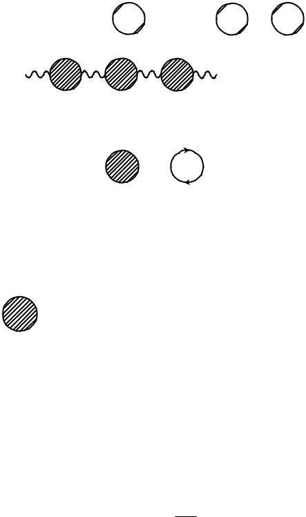
Gμυ= + +

+

+ . . .

Figure 3:

=

Figure 4:

This expression clearly diverges as ! 0. Before we show how to renormalize it let us discuss the meaning of (k). The full photon propagator is given by the series represented in Fig. 3, where

i (k) = sum of all one-particle irreducible

(2.36)

(proper ) diagrams to all orders

In lowest order we have the contribution represented in Fig. 4, which is what we have just calculated. To continue it is convenient to rewrite the free propagator of the photon (in an arbitrary gauge ) in the following form

iG0 =	g k2		! k2	+ k4		= P T k2	+	k4
		k k	1		k k	1	k k
	iG0T + iG0L							(2.37)

where we have introduced the transversal projector P T de ned by

P T = g	k k	!	(2.38)
	k2

obviously satisfying the relations,

8< k P T = 0

(2.39)

: P T P T = P T

9