8 - Chapman MATLAB Programming for Engineers

>>z1 = 3 + 4j;

>>z2 = z1 * exp(j*pi/2)

z2 =

-4.0000+ 3.0000i

>>z3 = j * z1

z3 =

-4.0000+ 3.0000i

>>theta1 = (180/pi) * angle(z1) theta1 =

53.1301

>>theta2 = (180/pi) * angle(z2) theta2 =

143.1301

>>theta_diff = theta2 - theta1 theta_diff =

90

Complex Conjugate. For every complex number z = x+jy = rejθ there is the complex conjugate

z = x − jy

Plotting z in the complex plane, by replacing y with −y , as shown in Figure 4.7, we see that the angle or phase of z is −θ. Thus,

Figure 4.7: Complex conjugate

z = x − jy = re−jθ

The mathematical procedure for finding a complex conjugate is to “replace j with −j ,” changing the sign of the imaginary part of the complex number.

For example:

67

>>z = 3 + 4j

z =

3.0000+ 4.0000i

>>zconj = conj(z) zconj =

3.0000- 4.0000i

>>theta = angle(z) theta =

0.9273

>>r = abs(z)

r =

5

>> zconj1 = r * exp(-j*theta) zconj1 =

3.0000- 4.0000i

Magnitude Squared: The product of z and its complex conjugate is

z z = (x − jy)(x + jy) = x2 + jxy − jxy − j2y2 = x2 + y2 = r2 = |z|2

or,

|z|2 = z z

and we see that the magnitude squared |z|2 is the product of z and its complex conjugate z .

For example:

>>z = 3 + 4j;

>>zz = conj(z) * z zz =

25

>>zmsq = abs(z)^2 zmsq =

25

Division: This operation is defined as the inverse operation of multiplication. The quotient z1/z2 is obtained in rectangular form by multiplying both the numerator and denominator of the quotient by the conjugate of z2:

z1	=		x1 + jy1
z2			x2 + jy2
	=		(x1 + jy1)(x2 − jy2)
			(x2 + jy2)(x2 − jy2)
	=		(x1 + jy1)(x2 − jy2)
			x2		+ y2
		2			2

68

=	x1x2 + y1y2		+ j	x2y1 − x1y2
	x2	+ y2
				x2	+ y2
	2	2	2		2

Division is more easily performed in exponential form

	z1	=	r1ejθ1
	z2		r2ejθ2
		=	r1ejθ1 e−jθ2
			r2ejθ2 e−jθ2
		=	r1	ej(θ1−θ2)
			r2

Thus, the magnitude of the quotient is the quotient of the magnitudes and the angle of the quotient is the di erence of the angle of the numerator and the angle of the denominator:

	z1		=	r1
				r2
z2

z1 = θ1 − θ2 z2

For example:

>>z2 = 2 + 1.5j

z2 =

2.0000+ 1.5000i

>>z4 = 1.25 + 2.5j

z4 =

1.2500+ 2.5000i

>>z1 = z4/z2

z1 =
1.0000+	0.5000i

>>magz2 = abs(z2) magz2 =

2.5000

>>magz4 = abs(z4) magz4 =

2.7951

>>magz1 = abs(z1) magz1 =

1.1180

>>magtest = magz4/magz2 magtest =

1.1180

>>argz2 = angle(z2) argz2 =

69

0.6435

>>argz4 = angle(z4) argz4 =

1.1071

>>argz1 = angle(z1) argz1 =

0.4636

>>ang_test = argz4 - argz2 ang_test =

0.4636

Algebraic Rules

The algebraic rules you have learned for real variables and numbers apply to complex variables and numbers.

Commutativity: Addition and multiplication can be done in either order without changing the result.

z1 + z2 = z2 + z1

z1z2 = z2z1

Associativity: Sums and products of three or more variables can be performed in sequential groups of two without changing the result.

(z1 + z2) + z3 = z1 + (z2 + z3)

(z1z2)z3 = z1(z2z3)

Distributivity: Multiplication can be distributed across a sum without changing the result.

z1(z2 + z3) = z1z2 + z1z3

Matlab Functions for Complex Numbers

To summarize, the following are the Matlab functions for complex numbers:

abs(z) Complex magnitude |z| (absolute value for real z) angle(z) Phase angle or argument of z

conj(z) Complex conjugate z imag(z) Complex imaginary part Im(z) real(z) Complex real part Re(z)

70

4.2.3Roots of a Quadratic Polynomial

In a previous example, we found that the roots of the quadratic polynomial

as2 + bs + c = 0

are given by:

b 1

s1,2 = −2a ± 2a b2 − 4ac

For the values of the coe cients considered in that example, the resulting roots were real. However, for other values of the coe cients, the roots can be complex. Having now reviewed complex numbers, we can investigate the problem of quadratic roots in more detail. There are three di erent cases for the solution, dependent on the value of the discriminant of the quadratic equation:

d = b2 − 4ac

• Overdamped (d > 0): Both roots are real and are given by

b 1

s1,2 = −2a ± 2a b2 − 4ac

The roots are located symmetrically about the point −b/2a. When b = 0, they are located

√

symmetrically about 0 at the points ±(1/2a) −4ac (in this case, −4ac > 0).

• Critically Damped (d = 0): The two roots are real and equal (we say they are repeated):

b s1,2 = −2a

•Underdamped (d < 0): The square root in the quadratic equation produces an imaginary number, so the roots are complex

			b		1
	s1,2 =	−		±					−(4ac − b2)
			2a		2a
			b			1
	=	−		± j						4ac − b2
			2 a			2a

Note that in this case, the roots s1 and s2 are complex conjugates:

s2 = s1

The roots are purely imaginary when b = 0

s1,2	=	±	j			c
						a

In Matlab, it is not necessary to determine which of the three cases applies to a given problem, as the square root function will appropriately return real or imaginary values as needed.

71

Example:

>>a=1; b=4; c=8;

>>x = -b/(2*a);

>>y = sqrt(b^2-4*a*c)/(2*a);

>>s1 = x + y

s1 =

-2.0000+ 2.0000i >> s2 = x - y

s2 =

-2.0000- 2.0000i

4.3Two-Dimensional Plotting

One of the major advantages of Matlab are its capabilities for displaying its results in the form of two-dimensional and three-dimensional graphics, providing what has come to be known as scientific visualization. In this section, Matlab capabilities are explained for producing two-dimensional plots in the context of the display of complex variables in the complex plane. In later sections, these two-dimensional graphics will be extended to other variables, in the context of the presentation of those variable types. For more information, type help graph2d.

Example: Plotting Complex Variables

The plot command can be used to plot complex variables in the complex plane. For example:

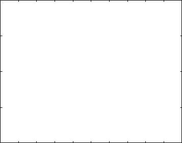
>>z = 1 + 0.5j;

>>plot(z,’.’)

This creates a graphics window, called a Figure window, named by default “Figure No. 1,” which becomes the active (top) window. The plot produced is shown in Figure 4.8, with z plotted as a point (due to the command ’.’) in the complex plane, with the real value (1.0) on the horizontal (x) axis and the imaginary value (0.5) on the vertical (y) axis. The axes have been scaled automatically, with a range of 0.0 to 2.0 on the horizontal axis and a range of -0.5 to 1.5 on the vertical axis. Numerical scales and tick marks have been added automatically.

This plot was exceedingly easy to produce, but it has many deficiencies that we can improve upon. Here are some improvements to consider:

•Control the scaling of the axes

•Produce a plot that is square instead of rectangular, having the same scale on both axes

•Include several complex variables on a single plot

72

1.5

1

0.5

0

−0.5

0

0.2

0.4

0.6

0.8

1

1.2

1.4

1.6

1.8

2

Figure 4.8: Simple plot of a complex number

•Label the axes

•Title the plot

•Label the plotted complex variables

The commands to implement each of these improvements will be introduced and discussed. The resulting plot produced by each command won’t be given, so you might try each of them in Matlab as you read this. Finally, when all of the commands have been discussed, a Matlab example session using them will be given and the results will be displayed.

4.3.12D Plotting Commands

For more information, type help graph2d.

Colors and Markers

Color and markers can be specified by giving plot an additional argument following the complex variable name. This optional additional argument is a character string (enclosed in single quotes) consisting of characters from the following table:

73

Symbol	Color	Symbol	Marker
y	yellow	.	•
m	magenta	o	◦
c	cyan	x	×
r	red	+	+
g	green	*
b	blue	s
w	white	d
k	black	v
		^
		<
		>	!
		p	"
		h	hexagram

Examples:

plot(z1,’b.’)	% plot variable z1				as a blue point
plot(z2,’go’)	%	plot	variable	z2	as	a	green circle
plot(z3,’r*’)	%	plot	variable	z3	as	a	red asterisk

Customizing Plot Axes

The axis command provides control over the scaling and appearance of both the horizontal and vertical axes of a plot. This command has many features, so only the most useful will be discussed here. For more complete information, refer to on-line help. The primary features are given in the following table

Command	Description
axis([xmin xmax ymin ymax])	Define minimum and maximum values of the axes
axis square	Produce a square plot instead of rectangular
axis equal	Equal scaling factors for both axes
axis normal	Turn o axis square, equal
axis(auto)	Return the axis to automatic defaults
axis off	Turn o axis background, labeling, grid, box, and tick
	marks. Leave the title and any labels placed by the
	text and gtext commands
axis on	Turn on axis background, labeling, tick marks, and,
	if they are enabled, box and grid

Adding New Curves

Using the hold command to add lines to an existing plot:

74

Command	Description
hold on	Retain existing axes, add new curves to current axes when new plot com-
	mands are issued. If the new data does not fit within the current axes limits,
	the axes are rescaled (for automatic scaling only)
hold off	Releases the current figure window for new plots
ihold	Logical command that returns 1 (True) if hold is on and 0 (False) if hold is
	o

Plot Grids, Axes Box, and Labels

There are several commands to control the appearance of the plot. These include:

Command	Description
grid on	Adds dashed grid lines at the tick marks
grid off	Removes grid lines (default)
grid	Toggles grid status (o to on, or on to o )
box on	Adds axes box, consisting of boundary lines and tick marks on top
	and right of plot
box off	Removes axes box (default)
box	Toggles box status
title(’text’)	Labels top of plot with text in quotes
xlabel(’text’)	Labels horizontal (x) axis with text in quotes
ylabel(’text’)	Labels vertical (y) axis with text in quotes
text(x,y,’text’)	Adds text in quotes to location (x,y) on the current axes, where (x,y)
	is in units from the current plot
gtext(’text’)	Place text in quotes with mouse: displays the plot window, puts up
	a cross-hair to be positioned with the mouse, and write the text onto
	the plot at the selected position when the left mouse button or any
	keyboard key is pressed

Printing Figures and Saving Figure Files

Plots can be printed using a figure window menu bar selection or with Matlab commands from the Command window.

To print a plot using commands from the menu bar, make the Figure window the active window by clicking it with the mouse. Then select the Print menu item from the File menu. Using the parameters set in the Print Setup or Page Setup menu item, the current plot is sent to the printer.

Matlab has its own printing commands that can be executed from the Command window. To print a Figure window, click it with the mouse or use the figure(n) command, where n is the figure number, to make it active, and then execute the print command:

>> print

% prints the current plot to the system printer

75

The orient command changes the print orientation mode, as follows:

Command	Description
orient portrait	Prints vertically in middle of page (default)
orient landscape	Prints horizontally, stretches to fill the page
orient tall	Prints vertically, stretches to fill the page
orient	Displays the current orientation

Options to the print command provide for writing the plot to a file in many di erent formats. For example, to write the plot as a PostScript format file in the current directory:

print -deps file

where file is the name of the file to be written, usually having the file name extension .ps to remind you that it is a PostScript file.

To view the contents of a PostScript file, type the following in a UNIX command window:

gv file

where file is the name of the PostScript file (including the .ps extension).

To print a PostScript file, type the following in a UNIX command window:

lp file

Refer to on-line help for the print command for further information on other file formats and options.

4.3.2Complex Plot Examples

Consider three examples to summarize the concepts of complex numbers, algebra, and geometry, plus the handling of complex numbers and plots by Matlab.

Rectangular Form Plot

The Matlab commands for a rectangular form plot:

z1 = 1.5 + 0.5j;

z2 = 0.5 + 1.5j;

z3 = z1 + z2;

z4 = z1 * z2;

z5 = conj(z1);

z6 = j * z2;

z7 = z2/z1; axis([-3 3 -3 3]); axis square;

grid on;

76